
Special Article - Biostatistics Theory and Methods
Austin Biom and Biostat. 2015;2(3): 1021.
Catchment Area Analysis Using Generalized Additive Models
Wheeler DC* and Wang A
Department of Biostatistics, Virginia Commonwealth University, USA
*Corresponding author: Wheeler DC, Department of Biostatistics, Virginia Commonwealth University, One Capitol Square, 830 East Main Street, Richmond,Virginia 23298-0032, USA.
Received: June 01, 2015; Accepted: June 11, 2015; Published: June 19, 2015
Abstract
A catchment area is the geographic area and population from which a health service center draws patients. Defining a catchment area allows the service center to describe its primary patient population and assess how well it meets the needs of patients within the catchment area. A catchment area definition is required for cancer centers applying for NCI-designated Cancer Center status. In this research, we estimated diagnosis catchment areas for the Massey Cancer Center (MCC) at Virginia Commonwealth University using a Generalized Additive Model (GAM) framework. We estimated diagnosis catchment areas for all cancers based on individual-level Virginia state cancer registry data. We used a GAM with a spatial smoother to model the residual log odds of being diagnosed with cancer at MCC after accounting for several covariates, including age, race, ethnicity, gender, and health insurance type. In addition, we used a Generalized Additive Mixed Model (GAMM) to account for multiple cancer diagnoses for the same patient. To define catchment areas, we identified the geographic areas with statistically significant residual log odds of being diagnosed for cancer at MCC. The diagnosis catchment area for MCC estimated from the GAM included 58 counties. Characteristics associated with increased odds of being diagnosed with cancer at MCC included black race, Hispanic ethnicity, younger age, no health insurance, and Medicaid health insurance.
Keywords: Catchment area; Generalized additive models; Cancer; Service area
Abbreviations
GAM: Generalized Additive Model; GAMM: Generalized Additive Mixed Model; TPRS: Thin Plate Regression Spline; TPS: Thin Plate Spline; GCV: Generalized Cross Validation; UBRE: Un- Biased Risk Estimator; P-IRLS: Penalized Iteratively Reweighted Least Squares; MCC: Massey Cancer Center; VCUHS: Virginia Commonwealth University Health System; VCR: Virginia Cancer Registry; NCI: National Cancer Institute; LAD: Local Authority District; SKCCC: Sidney Kimmel Comprehensive Cancer Center; NYCLIX: New York Clinical Information Exchange
Introduction
A catchment area is the geographic area and population from which a health service center draws patients. Defining a catchment area allows a health care facility to describe its primary patient population and assess how well it meets the needs of patients within the catchment area. A catchment area should capture a significant portion of the center’s patient activity and exclude areas whose contribution to center activity represents random variation. It should also reflect demographic and geographical influences on health center activity, including physical barriers to access and competition, and be proportional in geographic size to hospital size [1]. For cancer centers, a catchment area definition is required by the National Cancer Institute (NCI) when applying for NCI-designated Cancer Center status. According to the NCI, the catchment area must be based on geographically defined boundaries, such as census tracts or counties, and must include the local area surrounding the cancer center [2].
Several methods have been used in the literature to deterministically define a catchment area for a health care facility. Approaches focus on defining the catchment area using a threshold value for geographic distance, patient flow, or population size, where the geographic area found to be within the threshold composes the catchment area. For example, Luo and Qi [3] use a fixed distance (e.g., 30 miles) or a road network travel time to define a catchment area. Luo and Whippo [4] use a threshold-based population size to determine the distance for defining the catchment area. Alexandrescu et al. [5] define a catchment area by selecting areas that cumulatively account for 80% of hospital patients, and Phibbs and Robinson [6] define the catchment area based on the distance radius that contained 75% or 90% of hospital patients. Baker [7] selects spatial units that contained a threshold percent (e.g., 0.5%) of the total facility patient activity. The common drawback of these efforts is that the threshold is pre-specified and not estimated from the data.
Several different approaches have been used for estimating a catchment area from data. Judge et al. [8] use Thiessen polygons to define a catchment area, where the Thiessen polygon for the center comprises all points in space that are closest to that center than any other facility. This approach assumes that patients will travel to the facility that is closest in Euclidean space. A disadvantage of this approach is that it does not consider patient data when estimating the catchment area. Gilmour [1] uses K-means clustering to define a catchment area for the University College London Hospital in England based on three variables at the Local Authority District (LAD) level: the Euclidean distance between the hospital and a LAD, the proportion of the hospital admissions coming from each LAD, and the proportion of a LAD's total admissions going to the hospital. All LADs that provided at least one patient admission to the hospital of interest was considered in the K-means clustering. For the hospital of interest, the LAD data were divided into two clusters with K=2 clustering to define a catchment area for the hospital, where K-means clustering with K=2 effectively classifies each geographic unit as either in or out of the catchment area. An advantage of K-means clustering over the threshold approaches is that it estimates the geographic extent of the catchment area based on several variables at the area level. One shortcoming of the implementation of K-means clustering for catchment area delineation by Gilmour [1] is that it does not include patient-level covariates.
Another approach used for estimating a catchment area is the local spatial scan implemented in the software SaTScan [9]. The local spatial scan was created to detect geographic areas of statistically significantly elevated disease risk and can generally be used to detect a contiguous geographic area that differs statistically in some quantity from the surrounding area. Su et al. [10] use the local spatial scan statistic to estimate a catchment area for the Sidney Kimmel Comprehensive Cancer Center (SKCCC) at Johns Hopkins based on Johns Hopkins Hospital Cancer registry patient counts in counties in seven adjacent states and the District of Columbia. These authors use a Poisson model as the base for the local spatial scan to model the rate of SKCCC cancer patient counts per cancer death for each county. They define the rate with SKCCC cancer patient counts in the numerator and total cancer deaths as the denominator as a surrogate for the population with cancer. Onyile et al. [11] also use the local spatial scan with a Poisson model for estimating a catchment area for a health information exchange in NYC, the New York Clinical Information Exchange (NYCLIX), using patient and census data from the three adjacent states of New York, New Jersey, and Connecticut. The authors calculate the relative risk of visiting the NYCLIX facility through the rate of the number of NYCLIX patients in each county versus the number of people living in each county according to the 2010 US Census. One disadvantage of the local spatial scan for estimating catchment areas is that the analysis must be stratified to adjust for each covariate of interest, which is problematic for a large number of covariates. A limitation of the catchment area analysis of Su et al. [10] and Onyile et al. [11] is that the authors used hospital patient data and not state registry data, and hence the total cancer population in the area was unknown.
In more recent analysis, Wang and Wheeler [12] use a Bayesian hierarchical regression modeling approach to estimate catchment areas for the Massey Cancer Center (MCC) at the Virginia Commonwealth University Health System (VCUHS). Wang and Wheeler [12] aggregated Virginia Cancer Registry (VCR) patient data to the county level and adjusted for patient gender, age, and race with a Bayesian hierarchical logistic regression model with patient population strata. To estimate a diagnosis catchment area for MCC, the authors used exceedance probabilities to assess unusual clustering of patients going to MCC. An advantage of the approach of Wang and Wheeler is that Bayesian regression models estimate the catchment area stochastically from patient data through exceedance probabilities while adjusting for several covariates. One limitation of the analysis in Wang and Wheeler [12] is that it adjusted only for a small number of covariates aggregated to the county level. The models were limited in the number of population group strata due to the presence of patient counts of zero for some strata in certain counties.
As an alternative to the previous approaches, we propose to apply Generalized Additive Models (GAMs) and Generalized Additive Mixed Models (GAMMs) to estimate a diagnosis catchment area for the Massey Cancer Center at VCUHS. GAMs with spatial smoothing functions have been applied previously to model spatial variation of disease risk in several cancer studies [13-16]. The GAM framework is commonly used to determine geographic areas of significantly elevated risk for an event while adjusting for covariates. In this paper, we use a GAM to estimate a geographic area where the spatial odds of being diagnosed with cancer at MCC is significantly elevated while adjusting for many patient-level covariates. GAMMs effectively add random effects to GAMs to account for structured correlation among observations. The use of a GAMM is appropriate in this context due to the presence of multiple cancer diagnosis records for some patients in the registry data. As far as we know, this is the first use of GAMs and GAMMS to estimate a health center catchment area.
Materials and Methods
Study population
We obtained records from the Virginia Cancer Registry for all diagnosed cancer patients during years 2009-2011. The VCR data included demographic variables gender, race, ethnicity, age, health insurance type, reporting hospital, and residential location at the time of diagnosis or treatment. Originally, the data contained 160,307 records and 124,609 patients for the three years of study. We detected and deleted duplicated records for the same patient with the same cancer, tumor site, and diagnosed date, which was due to reporting of the same cancer for the same patient by different hospitals. After excluding duplicated records and records with missing values and patients living outside Virginia at time of diagnosis, we included 118,465 records and 112,565 patients in the analysis data set, where 5,559 patients had more than one cancer diagnosis. Of the total records in the analysis data set, 6,286 (5.3%) patients were diagnosed at Massey Cancer Center according to the reporting hospital coded in the VCR data.
Statistical modeling
We used the VCR cancer patient data to estimate a diagnosis catchment area for Massey Cancer Center during 2009-2011. We used a generalized additive model to model the odds of being diagnosed with cancer at MCC during 2009-2011. A GAM is a semi-parametric model extended from a generalized linear model and it has a general formula 12()
where is a link function, is a model intercept, and are smoothing functions of covariates for j=1,…,p, and is the error term [17]. The model allows nonlinear functions of covariates to be included in the regression equation and avoids restrictions imposed by parametric assumptions. GAMs can include functions with two or more dimensions, which makes them useful for spatial analysis. Specifically, for spatially referenced binary outcome data, GAMs can model the log odds of the event as a linear function of covariates and a spatial smoothing over geographic locations for i=1,…,n, as, 34()
where for presence of the event and for absence of the event, is a vector of linear regression coefficients representing the effects of covariates, and is a bivariate smoothing function. In our case, the event of interest is diagnosis of cancer at Massey Cancer Center.
We used a Thin Plate Regression Spline (TPRS) [18] as the smoothing function. A TPRS is a reduced rank version of the Thin Plate Spline (TPS), which is a type of penalized regression spline that provides knot-free locations. In general, a kth order spline is a piecewise polynomial function of degree k that is continuous and has continuous derivatives of orders 1,…, k at its knot locations. A regression spline fits a kth order spline with a set of knots at some specified locations. The performance of a regression spline depends on good selection of the knot locations, which is not trivial. A smoothing spline avoids the selection of knot locations by performing a regularized regression over the natural spline basis and placing knots at all the observed data points. There is a smoothing parameter that controls how smooth the spline is by shrinking away the wiggler basis functions as the parameter increases. A TPRS is a computationally convenient penalized regression spline that can include two covariates, making it ideal as a bivariate smoother over spatial coordinates. TPRS estimates parameters by minimizing the sum of squared error and a wiggliness penalty term. The objective function for TPRS fitting is , subject to 56()
with respect to vectors of coefficients and, where contains the first k columns of eigenvectors of the observed predictors, is a submatrix of diagonal matrix of eigenvalues, contains linearly independent polynomials, and is a smoothing parameter [18]. The smoothing parameter estimation problem is solved in the R package mgcv [19] by using Generalized Cross Validation (GCV) when the scale is unknown and using the Un-Biased Risk Estimator (UBRE) criterion when the scale is known. The model coefficients for GAMs with TPRS smoothers are estimated by maximizing the penalized likelihood function using a Penalized Iteratively Reweighted Least Squares (P-IRLS) algorithm. More details are available in [18].
To take into account multiple cancer diagnosis for some patients, we fitted a Generalized Additive Mixed Model (GAMM) with subjectlevel random effects. The GAMM model structure is 78()
where is a row of a random effects model matrix and is a vector of random effect coefficients with unknown positive definite covariance matrix with parameter. In our model, the random effect was included for each record i for subject j. The random effects added to a GAM are parametric terms penalized by a ridge penalty, which is equivalent to an assumption that the coefficients are independent and identically distributed normal random effects [18]. GAMMs are also implemented in the R package mgcv.
In the GAM and GAMM, we adjusted for several covariates that could be associated with odds of being diagnosed with cancer at MCC. The patient characteristics of race, gender, age, and health insurance status were included in the models. Specifically, we included in age at diagnosis; the gender variables male and other (hermaphrodite, transsexual, unknown) gender with female as the reference; the race variables black, other non-white race, and unknown race with white as the reference; Hispanic ethnicity with non-Hispanic ethnicity as the reference; and the health insurance variables of no insurance, self-pay, Medicaid, Medicare, other (TRICARE, military, Veterans Affairs, Indian/Public Health Service) insurance, and unknown insurance with private (managed care, HMO, PPO, or fee-for-service) insurance as the reference.
To estimate the catchment area from the models, we conducted a Monte Carlo assessment of the local significance of the spatial smooth term in the GAM and GAMM. The permutation procedure is based on Monte Carlo randomization of event labels and associated covariates while conditioning on the number and location of observed data points. Randomization of labels is consistent with the null hypothesis of constant risk of the event throughout the study area [20]. The model is fitted to each of 999 permuted data sets and then is used for prediction on a 50x50 grid that covers the study area. This builds a point wise distribution of the spatial smooth term under the null hypothesis at each grid cell. The spatial smooth prediction from the model for the observed data is then compared with the point wise distribution at each grid cell to identify areas with significantly elevated risk of the event. Specifically, the spatial predictions from the observed and permuted data are ranked in ascending order and significant risk areas are identified in this case by the points that have observed spatial log-odds that are above 95% of the ranked values of the point-wise permutation distribution. To create the catchment area map, we calculated the spatial intersection between the significant spatial grid cells and the counties in Virginia.
Results and Discussion
The odd of being diagnosed with cancer at Massey Cancer Center was associated with several variables (Table 1). The parameter estimates were very similar between the GAM and GAMM, with differences only in the fourth decimal place for two parameters (intercept and other race). Hence, accounting for multiple observations for some subjects had little effect on the estimates of regression relationships. Odds of being diagnosed with cancer at MCC was statistically significantly associated with all the included covariates except other race and male gender, which was marginally significant (p-value = 0.09). Covariates significantly associated with increased odds of being diagnosed at MCC included other gender, black race, Hispanic ethnicity, no health insurance, self-pay, Medicaid, and Medicare insurance. Covariates significantly associated with decreased odds of being diagnosed at MCC included age, unknown race, and other health insurance. The fits of the GAM and GAMM were the same, with both explaining 32.6% of the deviance.
![]()
    GAM
    GAMM


    Variable
    Coefficient
    Standard Error
    p-value
    Odds Ratio
    Coefficient
    Standard Error
    p-value
    Odds Ratio


    Intercept
    -2.6136
    0.0791
    <0.001
    -
    -2.6135
    0.0791
    <0.001
    -


    Age
    -0.0347
    0.0012
    <0.001
    0.9659
    -0.0347
    0.0012
    <0.001
    0.9659


    Male
    -0.0493
    0.0293
    0.093
    0.9519
    -0.0493
    0.0293
    0.093
    0.9519


    Other gender
    3.1554
    1.1672
    0.007
    23.4635
    3.1554
    1.1672
    0.007
    23.4629


    Black
    0.3786
    0.0325
    <0.001
    1.4603
    0.3786
    0.0325
    <0.001
    1.4602


    Other race
    0.1481
    0.1057
    0.161
    1.1597
    0.1482
    0.1057
    0.161
    1.1597


    Unknown race
    -0.7816
    0.1942
    <0.001
    0.4577
    -0.7816
    0.1942
    <0.001
    0.4577


    Hispanic
    0.7274
    0.0498
    <0.001
    2.0696
    0.7274
    0.0498
    <0.001
    2.0696


    No insurance
    1.4820
    0.0786
    <0.001
    4.4017
    1.4820
    0.0786
    <0.001
    4.4017


    Self-pay
    1.1581
    0.0754
    <0.001
    3.1838
    1.1581
    0.0754
    <0.001
    3.1838


    Medicaid
    0.8710
    0.0661
    <0.001
    2.3894
    0.8710
    0.0661
    <0.001
    2.3894


    Medicare
    0.2384
    0.0402
    <0.001
    1.2692
    0.2384
    0.0402
    <0.001
    1.2692


    Other insurance
    -1.1022
    0.1243
    <0.001
    0.3321
    -1.1022
    0.1243
    <0.001
    0.3321


    Unknown insurance
    -0.9095
    0.0866
    <0.001
    0.4027
    -0.9095
    0.0866
    <0.001
    0.4027
Table 1:  Parameter estimates and odds ratios from Generalized Additive Model (GAM) and Generalized Additive Mixed Model (GAMM) to estimate catchment area
for Massey Cancer Center.
The spatial component of the GAM and GAMM was highly significant (approximate p-value < 0.001). The catchment area for MCC estimated from the spatial model component comprises 58 counties (Figure 1). The large catchment area covers central and eastern Virginia. It stretches to the northern and eastern coasts of Virginia, but does not include the Eastern Shore. This geographic definition of the diagnosis catchment area is similar to a previous definition determined from a Bayesian hierarchical logistic regression model using exceedance probabilities for county random effects [12]. That catchment area comprised 54 counties, including the two Eastern Shore counties, but did not stretch as far north or southeast.
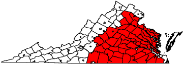
    Figure 1:  Virginia counties with Massey Cancer Center catchment area (red
fill) estimated from a GAM.
To compare cancer patient populations living inside and outside the MCC catchment area, we calculated summaries for certain patient characteristics inside and outside the estimated catchment area and stratified by diagnosis hospital (MCC vs. other) (Table 2). The summaries show that MCC patient population living inside the catchment area was younger and had greater proportions of women, blacks, Hispanics, patients with no insurance, patients who selfpay, and patients who used Medicaid compared with the patient population living inside the catchment area and diagnosed elsewhere. For example, the patient population diagnosed at MCC living inside the catchment area was 37.53% black, whereas the patient population diagnosed elsewhere and living inside the MCC catchment area was 25.10% black. Similarly, MCC patients living inside the catchment area were almost five times more likely to be uninsured (5.81%) compared with patients diagnosed elsewhere and living inside the catchment area (1.20%).
![]()
    Characteristic
    MCC Patient Inside    CA
    Non-MCC Patient    Inside CA
    MCC Patient Outside    CA
    Non-MCC Patient    Outside CA


    Age
    57.52
    64.91
    56.68
    63.4


    Male
    45.01%
    49.74%
    55.01%
    46.61%


    Black
    37.53%
    25.10%
    24.96%
    13.45%


    Other race
    1.93%
    1.38%
    3.56%
    4.30%


    Hispanic
    12.59%
    6.02%
    12.05%
    13.56%


    No insurance
    5.81%
    1.20%
    6.96%
    1.57%


    Self-pay
    5.51%
    1.51%
    6.28%
    2.28%


    Medicaid
    7.07%
    2.35%
    10.87%
    3.17%


    Medicare
    34.40%
    44.84%
    31.07%
    41.79%
Table 2: Cancer patient summary inside and outside estimated Catchment Area (CA) for Massey Cancer Center (MCC).
The MCC patient population living outside the catchment area was younger and more likely to be black (24.96%) compared with the patient population living outside the catchment area and diagnosed elsewhere (13.45%). Proportions of patients without health insurance, who self-pay, and used Medicaid were several times higher in the MCC patent population living outside the catchment area compared with the patient population living outside the MCC catchment area and diagnosed elsewhere. Comparing the MCC patient populations inside and outside the MCC catchment area, the patient population living inside the catchment area was more likely to be black (37.53% vs. 24.96%) and Hispanic (12.59% vs. 12.05%). Proportions of patients who were uninsured, self-pay or on Medicaid were higher in the MCC population living outside the catchment area. However, proportions of patients without health insurance or on Medicaid were greater outside the MCC catchment area than inside for both patients diagnosed at MCC and elsewhere.
Summaries of the underlying county populations according to 2010 US Census numbers stratified by catchment area status (inside vs. outside) reveal that the mean county proportion of blacks was much higher inside the catchment area (27.36%) than outside the catchment area (12.38%) (Table 3). As a measure of socioeconomic status, mean percent of homes that were vacant was slightly higher inside the catchment area (16.32%) than outside the area (16.16%).
![]()
    Characteristic
    County Inside CA
    County Outside CA


    Median Age
    41.04
    40.35


    Age 65+
    15.17%
    16.04%


    Male
    49.83%
    48.87%


    Black
    27.36%
    12.38%


    Hispanic
    3.78%
    5.00%


    Vacant Homes
    16.32%
    16.16%
Table 3:  County population characteristics from 2010 US Census inside and
outside Catchment Area (CA) for Massey Cancer Center.
Conclusion
In this paper, we used generalized additive models and generalized additive mixed models to estimate a diagnosis catchment area for Massey Cancer Center using state cancer registry data. We adjusted for patient age, gender, race, ethnicity, and health insurance status in both models. We also accounted for correlation in diagnosis records when subjects had multiple cancer diagnoses. Our results showed that the catchment area for MCC was quite large (n = 58 counties), which reflects the significant presence of this large, urban cancer center in Virginia. We also found that Massey Cancer Center serves a relatively large proportion of black, Hispanic, uninsured, self-pay, and Medicaid cancer patients. Blacks and Hispanics were significantly more likely to be diagnosed with cancer at Massey Cancer Center compared with whites and non-Hispanics, respectively. Cancer patients on Medicare and Medicaid and those with no health insurance or who self-pay were significantly more likely to be diagnosed with cancer at Massey Cancer Center when compared with patients with private health insurance. In addition to its significant presence, MCC appears to play an important role as a health care provider for traditionally underserved populations of cancer patients.
While GAMs have been used repeatedly in the disease mapping literature, the application of GAMs and GAMMs for estimating catchment areas is novel. Many of the existing methods for defining a catchment area are not probability-based or do not adjust for many covariates simultaneously. In contrast with other approaches for catchment area analysis, GAMs estimate the catchment area stochastically from the data and can also adjust for many covariates flexibly through splines. In addition, while we presented the catchment area estimate at the county level, any spatial scale could be used with individual patient data because we predicted the spatial log odds over a grid. The use of GAMs and GAMMs for estimating catchment areas should be applicable to other large hospitals, particularly when cancer registry data are available and covariate effects are of interest.
Acknowledgement
We gratefully acknowledge support from the Massey Cancer Center to conduct this study. We thank Cathy Bradley, Chris Gillam, Laurel Gray, Lynne Penberthy, and Valentina Petkov for assistance in acquiring the data used in this study.
References
- Gilmour SJ. Identification of Hospital Catchment Areas Using Clustering: An Example from the NHS. Health Serv Res. 2010; 45: 497-513.
- National Institutes of Health, National Cancer Institute, Office of Cancer Centers. Policies and Guidelines Relating to the P30 Cancer Center Support Grant. 2013; 1-56.
- Luo W, Qi Y. An Enhanced Two-step Floating Catchment Area (E2SFCA) Method for Measuring Spatial Accessibility to Primary Care Physicians. Health Place. 2009; 15: 1100-1107.
- Luo W, Whippo T. Variable Catchment Sizes for the Two-step Floating Catchment Area (2SFCA) Method. Health Place. 2012; 18: 789-795.
- Alexandrescu R, O'Brien SJ, Lyons RA, Lecky FE. A Proposed Approach in Defining Population-based Rates of Major Injury from a Trauma Registry Dataset: Delineation of Hospital Catchment Areas (I). BMC Health Serv Res. 2008; 8:80.
- Phibbs CS, Robinson JC. A Variable-radius Measure of Local Hospital Market Structure. Health Serv Res. 1993; 28: 313-324.
- Baker LC. Measuring Competition in Health Care Markets. Health Serv Res. 2001; 36: 223-251.
- Judge A, Welton NJ, Sandhu J, Ben-Shlomo Y. Geographical Variation in the Provision of Elective Primary Hip and Knee Replacement: The Role of Socio-demographic, Hospital and Distance Variables. Journal of Public Health. 2009; 31: 413-422.
- Kulldorff M. A Spatial Scan Statistic. Communications in Statistics: Theory and Methods. 1997; 26: 1481-1496.
- Su SC, Kanarek N, Fox MG, Guseynova A, Crow S, Ouabtadisum S. Spatial Analyses Identify the Geographic Source of Patients at a National Cancer Institute Comprehensive Cancer Center. Clinical Cancer Research. 2010; 16: 1065-1072.
- Onyile A, Vaidya SR, Kuperman G, Shapiro JS. Geographical Distribution of Patients Visiting a Health Information Exchange in New York City. J Am Med Inform Assoc. 2012; 20: 125-130.
- Wang A, Wheeler DC. Catchment Area Analysis using Bayesian Regression Modeling. Cancer Informatics. 2015; 14: 71-79.
- Webster T, Vieira V, Weinberg J, Aschengrau A. Method for Mapping Population-based Case-control Studies: An Application Using Generalized Additive Models. Int J Health Geogr. 2006; 5: 26.
- Vieira VM, Webster TF, Weinberg JM, Aschengrau A. Spatial-temporal Analysis of Breast Cancer in Upper Cape Cod, Massachusetts. Int J Health Geogr. 2008; 7: 46.
- Wheeler DC, De Roos AJ, Cerhan JR, Morton LM, Severson R, Cozen W, et al. Spatial-temporal Analysis of Non-hodgkin Lymphoma in the NCI-SEER NHL Case-control Study. Environ Health. 2011; 10: 63.
- Wheeler DC, Ward MH, Waller LA. Spatial-temporal Analysis of Cancer Risk in Epidemiologic Studies with Residential Histories. Annals of the Association of American Geographers. 2012; 102: 1049-1057.
- Hastie TJ, Tibshirani RJ. Generalized Additive Models. CRC Press. 1990.
- Wood SN. Generalized Additive Models: An Introduction with R. Chapman and Hall/CRC. 2006.
- Wood SN. Fast stable restricted maximum likelihood and marginal likelihood estimation of semiparametric generalized linear models. Journal of the Royal Statistical Society (B). 2011; 73: 3-36.
- Waller L, Gotway C. Applied Spatial Statistics for Public Health Data. Hoboken, New Jersey: John Wiley & Sons. 2004.