
Research Article
Austin Biom and Biostat. 2014;1(2): 7.
Penalized Likelihood Regression Approach for Quantitative Trait Loci Mapping From Samples with Related Individuals
Ku HC1 and Zhu L2*
1McDermott Center for Human Growth and Development, University of Texas Southwestern Medical Center, USA
2Department of Statistics, Oklahoma State University, USA
*Corresponding author: Zhu L, Department of Statistics, Oklahoma State University, 301C MSCS Bldg, Stillwater, 74078, USA.
Received: November 11, 2014; Accepted: December 04, 2014; Published: December 11, 2014
Abstract
Identifying Quantitative Trait Loci (QTL) by association mapping is critical for understanding the genetic architecture of complex traits or diseases. Many statistical methods have been developed to locate genes and estimate the effects of these genes that are responsible for quantitative traits. Penalized maximum likelihood method is one of the powerful statistical tools for QTL mapping, especially in dealing with the problem of p >n, where p is the number of genetic effects and n is the sample size. Most methods derived from it are limited to analyzing single trait from samples with independent individuals. Genetic inheritable complex diseases usually affect family members and are expressed by multiple correlated traits. The purpose of this study is to develop a statistical method (penalized likelihood regression approach) to target QTL from samples in a general setting, that is, arbitrary related individuals, for both single and multiple traits. Simulation studies show that the proposed method has great performance in detecting QTL in both single- and two-trait scenarios with related and unrelated individuals.
Keywords: Quantitative trait loci; Penalized maximum likelihood; Related individuals; Genome-wide association; False discovery rate; Multiple-trait association mapping
Introduction
Identifying Quantitative Trait Loci (QTL) is critical for understanding the genetic architecture of complex diseases or inheritable traits. Thus, QTL mapping aims to locate genomic variants and estimate the effects of these variants that are responsible for quantitative traits. One of initial methods for QTL mapping is Single Marker Analysis (SMA) based on a simple regression model [1,2]. The basic concept of this method is to consider each marker individually and check if there is an association between the trait and a marker. SMA provides the valuable framework for QTL mapping since the model is simple and easy to be extended to the multiplemarker analysis. However, this method tends to underestimate QTL effects and is not powerful unless sample size is relatively large [3]. Moreover, this method may not be able to detect the accurate position of QTL, as it is unlikely that QTL is right at the marker position if the density of markers does not cover all variants in the genome [4]. Interval Mapping (IM) method, an extension of SMA, was introduced by Thoday [5] and mathematically developed by Lander and Botstein [3]. IM can estimate the location and effect of QTL between two flanking markers if only one QTL on a tested region is assumed. The estimated location and effect of QTL are likely biased since the test statistics may be affected by other putative QTL out of the tested region. For multiple QTL methods, an extended and improved version of IM, called Composite Interval Mapping (CIM) [6-9] that accounted markers outside of the tested interval, has been widely applied in practice. The main idea of CIM is to combine IM with multiple regression analysis to detect multiple QTL. Some markers outside of the tested region are selected as genetic background to increase the resolution of IM. However, model-selection is somewhat subjective, depending on what variables are included or excluded [10- 13]. Moreover, for SNP datasets, the number of SNPs (p) is usually larger than the number of individuals (n), which makes the QTL mapping more challenging.
Bayesian shrinkage methods have become important computational tools to overcome the problems in CIM. Xu [14] proposed a method called Bayesian analysis implemented via the Markov Chain Monte Carlo (MCMC). In this model, individuals were assumed independent. Each marker was treated as a putative QTL and included in the model as one variable. The variance of QTL effects was then assumed to be different across QTL as a prior parameter. To perform satisfactorily, a sample size of 600 independent individuals is suggested in the method of Bayesian analysis implemented via the MCMC [15]. In addition, the MCMC algorithm requires a large number of iteration to converge to the stationary distribution. Both large numbers of sample size and iteration require intensive computational time, which becomes a major concern for the method. To reduce the computational burden, Zhang and Xu [16] developed an extended method of the Bayesian analysis implemented via the MCMC, called the penalized maximum likelihood method. It is similar in spirit to the method proposed by Xu [14] in that both methods shrink the null marker effects to zero, where the null marker effects are defined as the effects of the markers that are truly not QTL. The key of this method is to impose a prior normal distribution on the effect of each marker as a penalty, allowing the penalty to vary across each marker.
Both Bayesian shrinkage methods consider all markers simultaneously and include as many QTL as the model can handle. However, these methods assume independence among individuals and can only deal with one trait at a time. In addition, these methods ignore the issue of multiple tests, which result in an increased rate of overall type I error (i.e., false positive). Studies in humans, animals, or plants may involve related individuals such as trio families and inbred pedigrees. Furthermore, complex traits usually have multiple phenotypic measurements and these traits may be correlated. Statistical methods for QTL mapping that considering the relatedness among individuals as well as multiple traits are still under development. In this study, we propose extended penalized maximum likelihood methods for single- and multiple-trait analysis on arbitrary related individuals and retain the feature of handling the p >n problem. Multiplicity issue is also considered by selecting a threshold of LOD score that controls FDR at 0.05.
Methods
Single trait analysis
Let Zi denote the quantitative trait of individual i in an arbitrary pedigree and express as a linear function of the genetic effects. Assuming no interaction among effects, the model is
where b0> is the overall mean; p is the total number of markers; xij and wij are dummy variables indicating the genotype of the jth marker for individual i and defined as
for genotype A1A1, xij=0 and wij=1 for genotype A1A2, andfor genotype A1A2, such that they have a zero expectation and a unity variance [14]; bj and dj are additive and dominant effects associated with marker j, respectively. We assume bj and dj are independent; and ei˜N(0,s2) are the random environmental effect.
In the matrix form, when all characteristics of n individuals are included, formula (1) expands to
Z=1b1+X*B+W*D+E*, (2)
where Z is an nx1 vector of the quantitative trait; 1 is an nx1 vector of 1s; X* and W* are nxp matrices of dummy variables; and B and D are px1 vectors of additive and dominant effects, respectively.
We propose to take the relationship of individuals in a pedigree into account in the penalized maximum likelihood method by considering the relatedness coefficient ωω, which is defined as two times the kinship coefficient. The kinship coefficients of any arbitrary pedigree can be calculated based on the relationships between individuals. For instance, the relatedness coefficient for parentoffspring relationship is 0.5, meaning that theoretically 50% of the offspring's genome comes from that parent. Thus, in formula (1), we assume that Cov(eu,ev)=s2ωuv where ωuv is the relatedness coefficient for individual u and v. The distribution of E* for unrelated individuals is assumed to follow a multivariate normal distribution with mean vector 0 and covariance matrix s2In, where In is the nxn identity matrix.
When we take the relatedness among individuals into account, we assume E*˜N(0, s2Ω), where [Ω]uv=ωuv. Given the covariance matrix, it is possible to find a transformation matrix A [17] such that ATA=Ω-1 and the model then becomes Y=AZ=A1b0+AX*B+AW*D+AE*=Cb0+ XB+WD+E. Note that E˜N(0,s2In).
Suppose that θ = (b0,b1,...,bp,d1,...,dp,s2) is the vector of parameters of interest. Under the assumption of multivariate normality for the quantitative trait, the likelihood function of the pedigree is given by
where Φ is the normal density, β = Cb0+XB+WD, and
the main idea of penalty in the penalized maximum likelihood method is to have prior densities of the parameters, that is, hyper parameters, in the Bayesian framework. Since b0 and s2 are always in the model, their inclusion should not be penalized [16].
In this study, prior densities of parameters are defined similarly as Xu [14]. Assume that additive and dominant effects are normally distributed, then bj˜N(μbj,s2 bj) and dj˜N(μdj,s2 dj) for j = 1,..., p. The hyper parameters μbj, μdj, s2 bj and s2 dj in the prior distributions are very important in the oversaturated model, from the experience of Zhang and Xu [16] these parameters should be estimated from the data by assigning prior distributions to μbj and μdj such that μbj˜N(0, s2 bj /?) and μdj˜N(0, s2 dj /?) for j = 1,..., p, where ? is a positive prior value for accessing μbj and μdj. It is useful in the shrinking process because it controls the convergence rate.
Now suppose that ξ=(μb1,...,μbp,μd1,...,μdp,s2 b1,...,s2 bp,s2 d1,...,s2 dp) is the vector of the hyper parameters of interest in the prior distribution. The prior density is
and the penalized likelihood function is ψ(?,?)=L(?)P(?,?). The parameters in the penalized likelihood function are estimated by taking the derivative of logψ(?,?) with respect to ? and ? and then set the derivatives equal to zero. The solutions (PMLE) are performed by an iterative algorithm in the following steps.
Step 1. Initialization: set ?>0 and initialize ? and ? values
Step 2. Updating b0:
Step 3. Updating bj:
Step 4. Updating dj:
Step 5. Updating s2:
Step 6. Updating μbj:
Step 7. Updating μdj:
Step 7. Updating μdj:
Step 8. Updating s2bj:
Step 9. Updating s2dj:
Step 10. Repeat 2-9 until a certain criterion of convergence is satisfied. The terms for s=bj or s=dj, in Steps 3 and 4 are important in the iterative algorithm. s2 s's are defined in Steps 8 and 9 as the average of squared deviance and a squared mean effect multiplied by a constant. If s2 s is large (large effect), the estimated additive effect (bj) or dominant effect (dj) is expected to be unaffected (i.e. no shrinkage). However, if s2 sis small (small effect or no effect), the estimates will be shrunk towards zero.
Theoretically non-QTL effects are shrunk to zero whereas QTL with effects subject to no shrinkage. This makes the signals of QTL very clear. The estimated additive and dominant effects should be visualized by plotting the estimated effects over all markers along the genome. To ensure that the estimated effects are significant, a likelihood ratio test can be performed. Due to over parameterization, the usual likelihood ratio test is not appropriate. Therefore, we follow a two-stage process proposed by Zhang and Xu [16]. In the first stage, markers that have estimated effects are selected for the second stage of analysis. This is good because biologically we are not interested in the effects that are relatively small. In the second stage of analysis, since the dimension of markers is greatly reduced, a likelihood ratio test can be performed on the markers that have passed the first round of selection. To test the null hypothesis of no additive or dominant effects, we apply the LOD score test [3],
where j is the index of the marker after the first round of selection,
is the likelihood under the null hypothesis, and L(?) is the likelihood without restriction on the parameters. The null hypothesis is rejected if LODj exceeds a threshold that controls the FDR at 0.05.Multiple traits analysis
For studies that involve multiple traits (e.g. in clinics), singletrait model will simply ignore the correlation among these traits and detect QTL for each trait separately. However, complex traits, especially for complex diseases, these traits may be correlated. To analyze correlated traits in one model, we expect to gain more statistical power in detecting QTL. In this study, we also propose an algorithm that incorporates the correlation between traits in the model. This algorithm can be easily extended to a model with more than two traits. The definitions of notations in the two-trait model are similar to those in the single-trait model, except now they are 2x1 vectors. We distinguish notations for the two-trait model from the single-trait model by having underscores on matrices for the two-trait model. That is, let Zi=[Zi (1),Zi (2)]T be a 2x1 vector of quantitative traits (1) and (2) of individual i in a pedigree. The model is where 1 is a 2x1 vector of 1s; xij and wij are 2x1 vectors of dummy variables; bj and dj are additive and dominant effects associated with maker j, respectively; and ei is a 2x1 vector of the random environmental effect. Note that ei ˜N(0,s2R), R is a 2x2 correlation matrix with correlation coefficient r between two quantitative traits on the off- diagonal. In the matrix form, the statistical model can be expressed as Z=1b0+X*B+W*D+E, where W˜N(0,(Ω⊗s2R)) and ⊗ is the Kronecker product. Similar to the single-trait model, we use A as a transformation matrix such that Y=(A⊗I2) Z=Cb0+XB+WD+E and E˜N(0,(In⊗s2R)).
The likelihood function is
where now ?=(b0,b1,...,bp,d1,...,dp,r,s2), β=Cb0+XB+WD and i=Cibi+XiB+WiD. Note that b0 r, and s2 are not penalized. The prior density is the same as that in the single-trait analysis. The penalized log likelihood function is ψ(?,?)=L(?)P(?,?). The derivation of the maximum likelihood estimates for two-trait model is similar to the single-trait model with an additional step of updating r, the coefficient of correlation between two traits.
Step 1. Initialization: set ?>0 and initialize ? and ? values.
Step 2. Updating b0:
Step 3. Updating bj:
Step 4. Updating dj:
Step 5. Updating r:
E(1)=Y(1)-C(1)b0-X(1)B-W(1)D E(2)=Y(2)-C(2)b0-X(2)B-W(2)D r=corr(E(1),E(2)).Step 6. Updating s2:
Hyperparameters for two-trait model in Steps 7 to 10 are the same as Steps 6 to 9 in single-trait model.
Step 11. Repeat steps 2-10 until a certain criterion of convergence is satisfied.
We first choose candidate QTL with either in the first stage of analysis. In the second stage, we perform the likelihood ratio test with markers that have passed the first stage of selection. The LOD score test in formula (3) is then applied to check if there is significant additive or dominant effect at a given marker.
Controlling false discovery rate
Multiplicity issue is an important problem in testing many hypotheses simultaneously. In this study, we first took the commonly used threshold, LOD = 3, proposed by Morton [18], and found that 4 out of 24 scenarios that we explored in the single trait analysis and 13 out of 36 scenarios that we explored in the two-trait analysis had the Monte Carlo estimated FDRs greater than 0.05. We then tried the threshold of LOD = 3.3 as suggested by Lander and Kruglyak [19] and found that 3 out of 24 scenarios in the single trait analysis and 2 out 36 scenarios in the two-trait analysis with the estimated FDRs exceeded 0.05. Finally, when we used LOD = 3.5 as the threshold, the estimated FDRs in all scenarios in both single- and two-trait analysis are controlled at 0.05.
Simulation studies
We conducted computer simulations using Matlab software [20] to investigate the performance of the proposed methods. For singletrait model, 201 markers were simulated by SimPed program [21] with two levels of sample sizes, n = {150,300}. The Minor Allele Frequency (MAF) across all markers is assumed to be uniformly distributed, MAF ˜ Unif (0.1, 0.5). Markers were evenly spaced with 1cM between two adjacent markers and each marker was assumed to be associated with two parameters, an additive and a dominant effect. The number of parameters in the model (402 in total) was larger than the number of individuals (n). We explored and compared the performance of our proposed method at three levels of heritability (h2 = 0.4, 0.6, and 0.8) and four pedigree structures (I (a), II (b), III (a+b+c), and IV (d)), where pedigree structure IV could be considered as a family with inbred individuals that is commonly seen in animals or plants. These pedigree structures are illustrated in Figure 1.

Figure 1: Pedigree structures for simulation.
We assigned four QTL at various locations with their sizes of additive and dominant effects listed in Table 1. The genetic variance was calculated by summing all the variations across QTL, where b and d are the additive and dominant effect, respectively. The variance of the random environmental effect s2 is then determined by different levels of heritability.
    QTL
    Position (cM)
    Additive (b)
    Dominant (d)


    1
    40
    4
    2


    2
    80
    2
    1


    3
    120
    2
    0


    4
    160
    0
    2
Table 1: Locations and effects of the four QTL used in the simulation.
There are 24 (= 3x2x4) scenarios in total according to the combination of factors we explore in this study (3 levels of heritability, 2 levels of sample size, and 4 pedigree structures). These factors are summarized in Table 2. We are specifically interested in two questions: (1) how good are the estimates and statistical power? (2) Is the FDR under control? In order to answer these questions, we carry out simulation studies by using the Monte Carlo method. In this study, each scenario is replicated 500 times to evaluate the accuracy of the estimates and the statistical power. Our proposed methods are model-selection-free. Thus we expect it takes less number of iterations to converge compared with other model-selection based MCMC approaches. Moreover, all non-QTL effects are shrunk to zero, so we expect to have clear signals of QTL effects if QTL exist.
    Factor
    Value


    Heritability
    0.4,    0.6, 0.8


    Number of    individuals
    150,    300


    Pedigree structure
    I,    II, III, IV
Table 2: Factors and values used in the simulation studies of single-trait analysis.
Initially, we set bj=dj=??bj=sdj=0, s2 bj=s2 dj=1, b0=mean(Y), and s2 =Var(Y) for j = 1, 2,..., p. The convergence criterion is the norm at the tth iteration. The prior value η is set to be 5. Since η controls the convergence rate of the shrinking process, it is more sensitive with a smaller value at the cost of a slower convergence. For other values such as 10 and 20, we have verified that the results are consistent (results not shown). The test statistic LODj is calculated after this twostage process and the threshold used in the study is LODj ≥ 3.5, which is determined by controlling FDR at 0.05.
For two-trait analysis, we evaluate the performance of the method by using 150 individuals only with 500 replicates since increasing sample size should increase the power theoretically. The effects of different levels of heritability and structures of pedigree on the power of tests are also considered. Additionally, we also explore whether the proposed method is robust to any correlation between traits by considering three levels of correlation coefficient (r = 0.4, 0.6, and 0.8). These factors are summarized in Table 3. The QTL locations and sizes of their additive and dominant effects used for simulation are listed in Table 1. The prior value η and the convergence criterion are the same as defined in the single-trait analysis. Using formula (3), the test statistic LODj is calculated after the two-stage process. LODj= 3.5 is the criterion of rejection, which is determined by controlling FDR at 0.05.
    Parameter
    Value


    Heritability
    0.4,    0.6, 0.8


    Correlation    coefficient
    0.4,    0.6, 0.8


    Pedigree structure
    I,    II, III, IV
Table 3: Factors and values used in the simulation studies of two-trait analysis.
Simulation results
Single-trait analysis: The estimates of additive and dominant effects at each marker for all 24 scenarios are plotted in Figures 2 and 3, respectively. These estimates at each marker are obtained by averaging the estimated effects from 500 replicates. By the Bayesian shrinkage methods, the non-QTL effects shrink towards zero compared with visible peaks at QTL positions. Our data show that the estimates of non-QTL effects are very close to zero, which served as the background, providing extremely clear signals of QTL effects at true QTL locations.
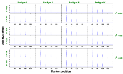
Figure 2 : The estimated additive effects against marker positions (singletrait).
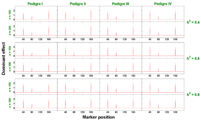
Figure 3: The estimated dominant effects against marker positions (singletrait).
The power is defined as the proportion of alternative hypotheses that are corrected rejected [22]. In this study, it is calculated by the number of QTL detected divided by the number of QTL assigned in the simulation. The estimates of average power of QTL detection across replicates for each of these 24 scenarios are compared and presented in Figure 4. As we expected, increasing sample size improves the power. Similarly, a higher heritability also results in a higher power in detecting QTL. For a relatively small sample size (n = 150) with a relatively low heritability (h2 = 0.4), the average power is moderate. It ranges from 48.1% to 52.8% for these four pedigree structures we explored. This power increases to a range from 76.2% to 82.8% with h2 = 0.6. It is significantly improved, reaching from 91.3% to 94.8% when the heritability is 0.8. Intuitively, this makes sense since a larger portion of phenotypic variation is explained by genetic variation with a higher heritability and therefore the larger effect is easier to be detected. For a large sample size (n = 300), the average power is at least 84% for all scenarios. In addition, the statistical power is not sensitive to pedigree structure, which demonstrates that our proposed method is robust and can be flexibly applied to QTL detection from arbitrary pedigrees.
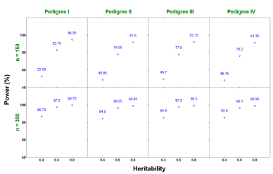
Figure 4: Power estimates under different scenarios from single-trait analysis.
As presented in Figure 4, the statistical power of our method for detecting QTL can be influenced by the magnitude of the heritability as well as sample size. To help researchers understand what sample size is needed in the study of QTL mapping with different levels of the heritability, we show how statistical power changes with the product of the heritability and sample size. We further explore 4 levels of the heritability (h2 = 0.2, 0.4, 0.6, and 0.8) and 6 levels of sample size (n = 150, 180, 210, 240, 270, and 300). The plot of statistical power versus the product of all combinations of the above levels of h2 and n is reported in Figure 5. We can see from this figure that the statistical power exponentially grows as the product of the heritability and sample size increases. When h2xn > 120, the statistical power of our method for detecting QTL reaches over 80%. That means if the trait has low heritability, say 0.2, we need to increase sample size to 600 in order to have a great power (80%) for the method to detect QTL. However, if h2 = 0.8, a sample of size 150 will be enough to reach the same power.
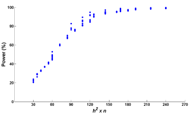
    Figure 5:  Power estimates under the product of the heritability and sample
size.
Two-trait analysis: Similar to the single trait analysis, we also evaluate the performance of our proposed two-trait penalized likelihood regression approach in all 36 (=3x3x4) scenarios (a combination of h2 ∈ {0.4, 0.6, 0.8}, r ∈ {0.4, 0.6, 0.8}, and 4 pedigree structures). We show in Figures 6 and 7 that the estimated additive and dominant effects for all scenarios have clear peaks at the QTL locations we assigned and non-QTL effects are close to zero. The estimated power of QTL detection is shown in Figure 8. With a low heritability (h2 = 0.4), the average power ranges from 54.9% to 68.3% across three levels of correlation coefficient and four pedigree structures. The power increases to a range from 84.3% to 90.6% with h2 = 0.6 and goes from 93.3% to 98% with h2 = 0.8. Compared with single trait analysis, the estimated power of QTL detection performs slightly higher in the two-trait analysis. As we expected, taking the correlation between traits and analyze them jointly gains more power than analyzing each trait separately.
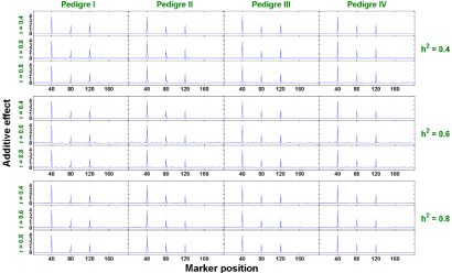
Figure 6: The estimated additive effects against marker positions (two-trait).
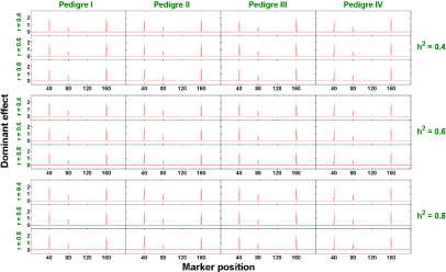
Figure 7: The estimated dominant effects against marker positions (two-trait).
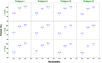
Figure 8: Power estimates under different scenarios from two-trait analysis.
Discussion
In this study, we propose two methods (single- and two-trait penalized likelihood regression models) to detect multiple QTL that are associated with multiple correlated traits while relaxing the assumption of independence among observations. Simulation study shows that both methods have moderate to great power in detecting QTL for traits with medium to high heritability. Although the power of detecting a QTL with a low minor allele frequency is not as good as we expected, the statistical power might be improved significantly by increasing the sample size.
As complex traits are usually measured by more than one trait, appropriate statistical models that can handle multiple traits simultaneously are currently under development but in a high demand, especially in the explosion of high-dimension data sets nowadays. The contribution of this study is to provide researchers an alternative and powerful approach for mapping QTL responsible for multiple correlated traits.
Although our proposed methods perform excellent in most of the common scenarios we explored, some challenges still exist. First of all, the choice of marker density for QTL mappings often decided by researchers. The decision of using a dense, sparse, or evenly spaced marker map may depend on the experimental costs or researchers' preference [23-26]. If only a sparse map is available, we suggest combining the proposed methods with an interval mapping method to increase the resolution of genetic markers and detect putative QTL within a tested region [27]. This will be an extension of penalized maximum likelihood method from marker-based mapping to interval mapping.
Moreover, our methods do not consider epistasis - interaction among genes and/or environment. One of the complications in modeling epistasis using an oversaturated model is the architecture among interaction components, such as types of interaction (gene by gene and gene by environment) and numbers of interaction. For instance, if there are 1000 markers and only two-way interactions are considered, the number of genetic effects would increase to around 500,000. Although penalized maximum likelihood method can handle different types of epistasis as well as large number of interaction, computational burden is still one of the major concerns. Further studies should focus on developing new statistical approach to handle this issue including the development of fast computational algorithms.
Finally, the proposed methods can provide clear peaks for large QTL effects, whereas shrink small QTL effects towards zero, which may result in the failure of detecting these small QTL effects. It is reasonable to ask whether small QTL effects can be excluded by shrinking these effects towards zero, even though small QTL effects are hard to detect [14]. Modification of proposed methods, such as incorporating a bias correction coefficient in the penalized maximum likelihood function [28], may be addressed to improve the power of QTL detection with small effects.
References
- Rebai A, Goffinet B, Mangin B. Comparing power of different methods for QTL detection. Biometrics. 1995; 51: 87-99.
- Soller M, Brody T, Genizi A. On the power of experimental designs for the detection of linkage between marker loci and quantitative loci in crosses between inbred lines. Theor Appl Genet. 1976; 47: 35-39.
- Lander ES, Botstein D. Mapping mendelian factors underlying quantitative traits using RFLP linkage maps. Genetics. 1989; 121: 185-199.
- Broman KW. Review of statistical methods for QTL mapping in experimental crosses. Lab Anim (NY). 2001; 30: 44-52.
- Thoday JM. Location of Polygenes. Nature. 1961; 191: 368-370.
- Jansen RC. Interval mapping of multiple quantitative trait loci. Genetics. 1993; 135: 205-211.
- Jansen RC, Stam P. High resolution of quantitative traits into multiple loci via interval mapping. Genetics. 1994; 136: 1447-1455.
- Zeng ZB. Theoretical basis for separation of multiple linked gene effects in mapping quantitative trait loci. Proc Natl Acad Sci USA. 1993; 90: 10972-10976.
- Zeng ZB. Precision mapping of quantitative trait loci. Genetics. 1994; 136: 1457-1468.
- Balding DJ, Carothers AD, Marchini JL, Cardon LR, Vetta A, Griffiths B, et al. Discussion on the meeting on 'Statistical modeling and analysis of genetic data'. Journal of the Royal Statistical Society: Series B-Statistical Methodology. 2002; 64: 737-775.
- Broman KW, Speed TP. A model selection approach for the identification of quantitative trait loci in experimental crosses. Journal of the Royal Statistical Society: Series B-Statistical Methodology. 2002; 64: 641-656.
- Kadane JB, Lazar NA. Methods and criteria for model selection. Journal of the American Statistical Association. 2004; 99: 279-290.
- Sillanpaa MJ, Corander J. Model choice in gene mapping: what and why. Trends Genet. 2002; 18: 301-307.
- Xu S. Estimating polygenic effects using markers of the entire genome. Genetics. 2003; 163: 789-801.
- Xu S. An empirical Bayes method for estimating epistatic effects of quantitative trait loci. Biometrics. 2007; 63: 513-521.
- Zhang YM, Xu S. A penalized maximum likelihood method for estimating epistatic effects of QTL. Heredity (Edinb). 2005; 95: 96-104.
- Cochrane D, Orcutt GH. Application of Least Squares Regression to Relationships Containing Auto correlated Error Terms. Journal of the American Statistical Association. 1949; 44: 32-61.
- Morton N. Sequential tests for the detection of linkage. Am J Hum Genet. 1955; 7: 277-318.
- Lander E, Kruglyak L. Genetic dissection of complex traits: guidelines for interpreting and reporting linkage results. Nat Genet. 1995; 11: 241-247.
- Math Works. MATLAB version 7.9. Natick, MA. The Math Works Inc. 2009.
- Leal SM, Yan K, Muller-Myhsok B. SimPed: a simulation program to generate haplotype and genotype data for pedigree structures. Hum Hered. 2005; 60: 119-122.
- Benjamini Y, Hochberg Y. Controlling the False Discovery Rate - a Practical and Powerful Approach to Multiple Testing. Journal of the Royal Statistical Society: Series B-Methodological. 1995; 57: 289-300.
- Darvasi A, Soller M. Optimum spacing of genetic markers for determining linkage between marker loci and quantitative trait loci. Theor Appl Genet. 1994; 89: 351-357.
- Hayes PM, Liu BH, Knapp SJ, Chen F, Jones B, Blake T, et al. Quantitative Trait Locus Effects and Environmental Interaction in a Sample of North-American Barley Germ Plasm. Theoretical and Applied Genetics. 1993; 87: 392-401.
- Kennard WC, Slocum MK, Figdore SS, Osborn TC. Genetic analysis of morphological variation in Brassica oleracea using molecular markers. Theor Appl Genet. 1994; 87: 721-732.
- van Der Schaar W, Alonso-Blanco C, Leon-Kloosterziel KM, Jansen RC, van Ooijen JW, Koornneef M. QTL analysis of seed dormancy in Arabidopsis using recombinant inbred lines and MQM mapping. Heredity (Edinb). 1997; 79 : 190-200.
- Guo Z. Novel method for increasing efficiency of quantitative trait locus mapping [dissertation]. Kansas State University, Manhattan, Kansas, 2007.
- Zhang J, Yue C, Zhang YM. Bias correction for estimated QTL effects using the penalized maximum likelihood method. Heredity (Edinb). 2012; 108: 396-402.