Kao-Tai Tsai; Karl E. Peace

Special Article - Biostatistics Theory and Methods

Austin Biom and Biostat. 2015;2(3): 1025.

Joint Modeling of Treatment Effect on Time-to-Event Endpoint and Safety Covariates in Control Clinical Trial Data Analysis

Kao-Tai Tsai* and Karl E. Peace

JPHCOPH, Georgia Southern University, USA

*Corresponding author: Kao-Tai Tsai, JPHCOPH, Georgia Southern University, Statesboro, GA 30458, USA

Received: June 01, 2015; Accepted: June 11, 2015; Published: July 09, 2015

Abstract

It is a common practice to perform a separate analysis of efficacy and safety data from clinical trials to estimate the benefit and risk aspects of a particular treatment regimen. However, by doing so, one is likely to miss the complete picture of the treatment effect given that these data are generated from the same study subjects and therefore most likely will be correlated. Therefore, it is desirable to analyze these data jointly to obtain a more complete profile of the treatment regimen. A substantial number of statistical methodologies have been proposed in the last decade to model the time-to-event data and longitudinal repeated measures jointly. These methods provide better insights to understand the treatment effect in time-to-event data by incorporating the information contained in the longitudinal repeated measures. In this article, we utilize the joint model method to analyze the time-to-event data, such as patient overall survival, and the repeated measures of laboratory test data to better estimate the treatment effect of a regimen. The data from a recent oncology clinical trial is used to illustrate the application of our proposed method.

Keywords: Joint modeling; Time-to-event data; Longitudinal repeated measures; Controlled clinical trials

Introduction

During the course of a clinical trial, several types of data are usually collected. This includes data to investigate the efficacy of the intervention of a test drug, the demographic data of the subjects under study, the laboratory data to understand the pharmacological effect of the treatment on the body, and the possible adverse effects, etc. Conventionally, it is common practice to analyze the efficacy and safety data separately to estimate the benefit and risk aspects of the treatment regimen. However, by performing separate analysis, one is likely to miss the complete picture of the treatment effect given that these data are generated from the same study subjects and therefore most likely will be correlated.

For example, in cancer clinical trials to study patient survival after treatment, patients are usually given treatment which can substantially cause neutropenia, namely, the reduction of white blood cells. Severe neutropenia can lead to infection or sepsis which can in turn lead to other complications that affect patient’s survival. This indirect treatment effect usually is not captured during the efficacy analysis alone. Therefore, it is more desirable to analyze these data together to obtain a more complete profile of the treatment regimen. Similar strategies have also been implemented in the study of HIV, neuroscience, and prostate cancers, just to name a few. In the following, we will focus our attention on the analysis of survival data and repeated measures of laboratory parameters such as white blood cell counts and other adverse effects.

A substantial number of statistical methodologies have been proposed in the last decade to model the time-to-event data and longitudinal repeated measures jointly. For example, Tsiatis et al. [1] in the study of AIDS, Diggle [2] in the study of patients with schizophrenia symptoms, Henderson, et al. [3] studied the positive and negative symptom scale in neuroscience, and Law et al. [4] in the study of disease progression biomarkers, etc.

Using parametric or semi-parametric maximum likelihood or and Bayesian methods, these authors estimated the parameters for both the longitudinal and event processes and used the associated asymptotic properties of the estimates. They also showed that the estimates from the joint model can usually be more efficient than the estimates from the separate models.

In this article, we utilize the joint model method to analyze the patient overall survival incorporating the laboratory data of neutrophils counts to better estimate the treatment effect of an experimental cancer therapy. We describe the statistical methodologies about joint modeling in section 2 followed by the parameter estimation and model diagnostics in section 3. In section 4, we illustrate the applications of these methods to the data from a recent cancer drug study. We conclude our paper with discussion in section 5.

Joint Modeling Methods

Let Ti denote the observed failure time for the i-th subject (i=1,…,n), which is taken as the minimum of the true event time $δ_{i} = I (T_{i}^{*} < C_{i})$ and the censoring time C_i, namely, $T_{i} = m i n (T_{i}^{*}; C_{i})$ . Furthermore, we define the event indicator as $δ_{i} = I (T_{i}^{*} < C_{i})$ , where I(.) is the indicator function that takes the value 1 if the condition $T_{i}^{*} < C_{i}$ is satisfied, and 0 otherwise. Thus, the observed data for the time-to-event outcome consist of the pairs {(Ti,{(Ti,di),i=1,…,n}.

For the longitudinal responses, let y_i(t) denote the value of the longitudinal outcome at time point t for the i-th subject. We should note here that we do not actually observe y_i(t) at all time points, but only at the very specific occasions t_ij at which measurements were taken. Thus, the observed longitudinal data consists of the measurements y_ij={y_i(t_ij), j=1,…,n_i}.

As in many clinical trials, data could be measured with errors due to the limitation of instruments and quantifications. That is especially true for the laboratory data. Therefore, as a general setting, we assume the following relationship between the observed value y_i(t) and the true underlying unobserved value m_i(t):

y_i(t) =m_i(t)+ε_i, (1)

where ε_i is the random error following a continuous distribution function. In the following, we will assume ε_i follows a normal distribution for simplicity.

For the event process, we assume the following hazard model:

$h_{i} (t | w_{i}) = h_{0} (t) \exp {γ^{'} w_{i}}, (2)$

where wi is the vector of covariates. One of our aim is to associate m_i(t) with the event outcome T_i in addition to the vector of covariates wi to better estimate the endpoints of interest.

To quantify the effect of m_i(t) on the risk for an event, a commonly adopted approach is to use a relative risk model proposed by Therneau and Grambsch [5]:

$h_{i} (t | M_{i} (t), w_{i}) = h_{0} (t) \exp {γ^{'} w_{i} + α m_{i} (t)}, (3)$

where M_i(t)={m_i(u),0<u<t) denotes the history of the true unobserved longitudinal process up to time t, h₀(.) denotes the baseline risk function, and wi is a vector of baseline covariates (such as a treatment indicator, history of diseases, etc.) with a corresponding vector of regression coefficients.

In the model above, the parameter a quantifies the effect of the underlying longitudinal outcome to the risk for an event in an additive manner; for instance, in the example section below, a measures the effect of the value of Absolute Neutrophils Counts (ANC) on the risk for death due to the fact that a low ANC value is likely to lead to infection which can indirectly cause medical complications to affect the overall patient survival.

The baseline risk function h₀(.) is typically left unspecified. However, within the joint modeling framework, Hsieh, et al. [6] had noted that unspecified h₀(.) can lead to underestimated standard errors of the parameter estimates. To avoid this problem, one can specify the function using the Weibull [7], Gamma, or for more flexible models in which h₀(.) is approximated using step functions or spline-based approaches. Alternatively, if the proportionality assumption in (2) or (3) fails, one can use the accelerated failure time model.

In order to incorporate a time dependent covariate within this framework, we define the survival function S_o as

$S_{0} ~ \int_{0}^{T^{*}} \exp {γ^{T} w + α m (s)} d s, (4)$

with the corresponding hazard function for subject i being

h_i(t|M_i(t),w_i)=h₀{V_i(t)}exp{_Tw_i+am_i(t)} (5) where

$V_{i} (t) = \int_{0}^{T^{*}} \exp {γ^{T} w_{i} + α m_{i} (s)} d s . (6)$

An important difference between equations (5) and (3) is that in the former the entire covariate history M_i (t) is assumed to influence the subject-specific risk (due to the fact that h₀(.) is evaluated at V_i(t), whereas in the latter the subject-specific risk depends only on the current value of the time-dependent covariate m_i(t). The survival function for a subject with covariate history m_i(t) equals S_i{t|M_i(t)}=S₀{V_i(t)}, which means that this subject ages on an accelerated schedule V_i(t) compared to S₀.

Equation (1) is a general framework of the relationship between the observed and true underlying data. The model needs to be explicitly specified during the data analysis to take into account the intermittent nature of the data collection. Namely, for subject i, one only observes y_ij={y_i(t_ij), j=1,…,n_ij} at a set of time {t_ij=1,…,n_ij}.

Assuming the normal error distribution and linear mixed effects model to describe the subject-specific longitudinal process, we have

y_i(t_ij)= m_ij(t_ij)+ε_ij(t_ij) $= x_{i}^{T} (t_{i j}) β + z_{i}^{T} (t_{i j}) b_{i} + ε_{i} (t_{i j}), ε_{i} (t_{i j}) ~ N (0, σ^{2})$ where β denotes the vector of the unknown fixed effects parameters, b_i denotes a vector of random effects, x_i(t) and z_i(t) denote row vectors of the design matrices for the fixed and random effects, respectively, and ε_i(t) is the measurement error term, which is assumed to be independent of b_i and with mean 0 and variance σ².

Parameter estimation and model diagnostics

Several estimation methods had been proposed for the joint modeling, e.g., semiparametric maximum likelihood (Hsieh, et al. [6]; Henderson, et al. [3]; Wulfsohn and Tsiatis [8], Tsiatis and Davidian [9]) and Bayes methods (Chi and Ibrahim [10]; Brown and Ibrahim [11]; Wang and Taylor [8]; Xu and Zeger [12]).

Briefly, the maximum likelihood estimation for joint models is based on the maximization of the likelihood corresponding to the joint distribution of the time-to-event and longitudinal outcomes {T_i,δ_i,y_i}. Since the time-independent random effects b_i underlies both the longitudinal and survival processes, assume

$f (T_{i}, δ_{i}, y_{i} | b_{i}, θ) = f (T_{i}, δ_{i} | b_{i}, θ) f (y_{i} | b_{i}, θ) (8)$

with

$f (y_{i} | b_{i}, θ) = \prod_{j} f {y_{i} (t_{i j}) | b_{i}, θ}, (9)$

where $θ = {(θ_{t}^{'}, θ_{y}^{'}, θ_{b}^{'})}^{'}$ denotes the parameter vector, with θ_t denoting the parameters for the event time outcome, θ_y the parameters for the longitudinal outcomes, and θ_b the unique parameters of the randomeffects covariance matrix, and f(.) denotes an appropriate probability density function for the longitudinal or event process.

Under the modeling assumptions and the conditional independence assumptions in equation (8), assume f{y_i(t_ij)|(b_i,θ_y} being the univariate normal density for the longitudinal responses, and f(b_i,θ_b being the multivariate normal density for the random effects, the joint log-likelihood contribution for the i-th subject is

$\log f (T_{i}, δ_{i}, y_{i}, θ) = \log \int^{} f (T_{i}, δ_{i} | b_{i}, θ_{t}, β) [\prod_{j} f {y_{i} (t_{i j}) | b_{i}, θ_{y}}] f (b_{i}, θ_{b}) d b_{i}, (10)$

where the likelihood of the event process is

$f (T_{i}, δ_{i} | b_{i}, θ_{t}, β) = {h_{i} (T_{i} | M_{i} (T_{i}), θ_{t}, β)}^{δ_{i}} S_{i} (T_{i} | M_{i} (T_{i}), θ_{t}, β), (11)$

with h_i(.) given by either (3) or (5), and

$S_{i} (t | M_{i} (t), w_{i}, θ_{t}, β) = \Pr (T_{i}^{*} > t | M_{i} (t), w_{i}, θ_{t}, β)$ $= \exp {- \int_{0}^{t} h_{i} (s | M_{i} (s), θ_{t}, β) d s} . (12)$

Since the integration in (10) generally has no analytical form, the maximization of the log-likelihood function (10) with respect to θ is conventionally performed using numerical integration techniques such as Gaussian quadrature and Monte Carlo. These approaches have been successfully applied in the joint modeling framework by various authors mentioned previously.

Residual plots are the conventional methods for model diagnostics to verify the appropriateness of the distributional assumptions and the adequacy of the model assumed. Model diagnostics for linear mixed model and time-to-event model have been well studied in the literature. However, given the inter-dependency between the longitudinal process and the event process, extra cautions are needed on the diagnostics for the joint model. For example, when a subject is discontinued the study or died, the data for either process will no longer be available.

When the process of subject discontinuation is random, the residuals may be less affected than the scenarios when the discontinuation was influenced by the failure of treatment and causes informative missing data issues. Rizopoulos, et al. [13] proposed a method to augment the observed data with randomly imputed longitudinal responses. Briefly, based on the parameter estimates of the joint model with available data, they performed multiple imputation with repeated sampling from the posterior distribution of the missing observations given the observed data. The complete profile of the longitudinal data can thus be established for each subject. The advantage of using the simulated values together with the observed data to calculate residuals is that these residuals inherit now the properties of the complete data model, and therefore they can be directly used in diagnostic plots.

Example

In this section, we present an example from a recent clinical trial to illustrate the use of the procedures described above. This is a multicenter clinical trial to investigate the treatment effect of an experimental medicine on breast cancer. Patients were randomized into two groups, treatment and placebo, to study the treatment benefit in disease progression. During the trial, the patients’ laboratory data on Absolute Neutrophils Counts (ANC) were also collected at each treatment visit to monitor the level of neutrophils. Low level of neutrophiles can possibly cause infection and lead to other complications to affect the patient disease. Even though the primary endpoint of the study is the treatment effect on disease progression which is usually estimated using efficacy data only, it is more informative to understand how the safety aspects of the study can also contribute to the patient’s disease progression.

The longitudinal ANC data was analyzed using a linear mixed effect model with a random intercept and fixed treatment and visit effects. Since the LME model requires the normality assumption, data was transformed using the Box-Cox power function to conform to the normality assumption. The normal plot after the transformation is shown in Figure 1.

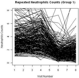
Figure 1: Box-Cox transformation of ANC values.

    
    
    Figure 1:  Box-Cox transformation of ANC values.

A total of 455 patients were randomized into two treatment groups (Group 1 and Group 3) in approximately 2:1 ratio with 204 events of disease progression and a total of 1745 repeated measures of ANC at the end of the study. Some patients had missing measures of the ANC during the duration of the clinical study. The patterns of the ANC values during the visits for each study are shown in Figure 2 and Figure 3, respectively. The boxplots for the treatments by visits are also shown in Figure 4. One can easily see substantial ANC values by treatment interactions during the course of the study. Therefore, we postulate a model for the longitudinal data to include the treatment, visit, and their interaction effects.

Figure 2: ANC level of Group 1.

    
    
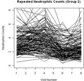
    Figure 2:  ANC level of Group 1.

Figure 3: ANC level of Group 3.

    
    
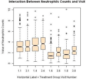
    Figure 3:  ANC level of Group 3.

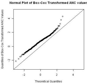
Figure 4: ANC values by treatment and visit.

    
    
    Figure 4:  ANC values by treatment and visit.

The Kaplan-Meier curves of survival times for the treatment groups is displayed in Figure 5. As common practice, a Cox proportional model was utilized to analyze the event data. Prior to performing the modeling, the assumption of proportionality was tested and the result is shown in Figure 6. The proportionality assumption on treatment effect seems to be reasonable judging from the graph.

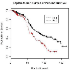
Figure 5: Kaplan-Meier curve of patient survival data.

    
    
    Figure 5:  Kaplan-Meier curve of patient survival data.

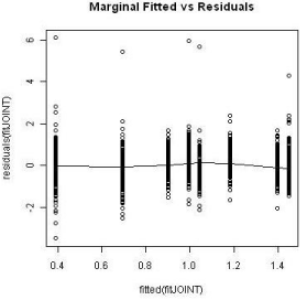
Figure 6: Proportional hazard test for treatment.

    
    
    Figure 6:  Proportional hazard test for treatment.

The REML estimates of the mixed effect model with fixed treatment, visit, treatment by visit interaction effects and random intercept are shown in Table 1. The results indicate both significant visit and interaction effects on the values of ANC.

Table 1: LME model of ANC with interaction.




  
    Covariate
    Value
    Std.Error
    DF
    t-value
    p-value
  
  
    (Intercept)
    1.5961
    0.0463
    1288
    34.419
    0.000
  
  
    trt3
    -0.1341
    0.0801
    453
    -1.673
    0.095
  
  
    visit
    -0.1520
    0.0069
    1288
    -21.821
    0.000
  
  
    trt3:visit
    0.0824
    0.0120
    1288
    6.820
    0.000



Table 1:  LME model of ANC with interaction.

Similarly, the estimate from Cox proportional hazard model with treatment as covariate indicates a highly significant treatment effect as shown in Table 2.

Table 2: Estimate of cox proportional hazard model.




  
    Covariate
    coef
    exp(coef)
    se(coef)
    z
    Pr(>|Z|)
  
  
    trt3
    0.5869
    1.7983
    0.1443
    4.068
    4.74e-05



Table 2:  Estimate of cox proportional hazard model.

After the separate LME model on the longitudinal data of ANC values and Cox proportional hazard model on the event data was fitted, a joint model was fitted using MLE to both the longitudinal and event sub-models and the results are shown in Tables 3 & 4.

Table 3: Estimates of the longitudinal process.




  
    Covariate
    Value
    Std.Err
    z-value
    p-value
  
  
    (Intercept)
    1.6008
    0.0460
    34.7970
     
  
  
    trt3
    -0.1312
    0.0809
    -1.6207
    0.1051
  
  
    visit
    -0.1515
    0.0071
    -21.3088
     
  
  
    trt3:visit
    0.0803
    0.0127
    6.3020



Table 3:  Estimates of the longitudinal process.

Table 4: Estimates of the event process.




  
     Covariate
    Value
    Std.Err
    z-value
    p-value
  
  
    trt3
    0.7340
    0.2544
    2.8855
    0.0039
  
  
    a 
    -0.0380
    0.0534
    -0.7112
    0.4769



Table 4:  Estimates of the event process.

The treatment effect (0.734) in Table 4 from the joint model is larger than that in Table 2 (0.586) from the Cox model alone. The value of α in Table 4 has a negative value which reduces the hazard for the patients with higher values of ANC, even though the effect of α did not reach the 5% significance level. Putting these findings together, one can conclude that the treatment effect on ANC indirectly affected patient survival. This incremental treatment would not have been detected if one were to analyze the treatment efficacy using only the survival data without bringing in the effect from ANC.

To assess the goodness of fit of the proposed model and better understand the differences between the treatment groups, we examined the difference of the random intercepts and the residuals from the fitted model for the groups. The random intercepts for the groups were plotted using a Q-Q plot as shown in Figure 7. The distributions appear to be similar between these two groups with a minor difference in locations; however, this difference does not seem to be significant.

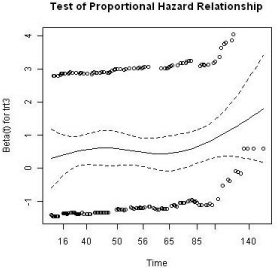
Figure 7: Comparison of random effects between groups.

    
    
    Figure 7:  Comparison of random effects between groups.

The subject-specific residuals $(r_{i} (t_{i j}) = y_{i} (t_{i j}) - x_{i} (t_{i j}) \hat{β} - z_{i} (t_{i j}) {\hat{b}}_{i})$ and marginal residuals $(r_{i} = y_{i} - x_{i} \hat{β})$ were plotted against the respective fitted values (Figures 8 and 9). The residuals did not seem to have any obvious pattern to suspect a lack-of-fit of the proposed model except for a minor dip in the left hand side of the subjectspecific residual plot. This could possibly due to the early dropouts of some patients who had severe disease at the entry of the clinical study. An imputation to ‘re-create’ the missing longitudinal data for these scenarios was conducted and the residual plot after the imputation seems to alleviate this downward dip to a few degrees but without substantial difference.

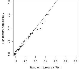
Figure 8: Comparison of random effects between groups.

    
    
    Figure 8:  Comparison of random effects between groups.

Figure 9: Comparison of random effects between groups.

    
    
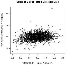
    Figure 9:  Comparison of random effects between groups.

Discussion

Medical intervention can usually produce effects in more than one aspect. They can be direct effect, such as patient survival in our example, which can be measured directly. They can also be indirect effects, such as the changes of ANC values in our example, which were affected by treatment and, in turn, affect the outcomes of interest such as patient survival. The joint analysis of direct and indirect effects to assess the intervention efficacy has been well demonstrated in psychiatric research and other related scientific areas. In other words, to better understand the complete profile of the treatment effects, data needs to be analyzed in more than one aspect.

It is a common practice in clinical trials to estimate the treatment effect using the efficacy data, with a limited number of covariates, because that is a most direct and conventional approach to gauge the effect. However, this kind of limited data analysis can sometimes miss the more complete picture of how the treatment really works. In conventional clinical trial data analysis, efficacy and safety data are usually analyzed separately. However, as we have shown in this article, joint analysis of these variables can reveal extra information about the treatment and lead to a better understanding of the treatment effect, which cannot usually be shown by the separate analysis.

Statistical methodologies in joint modeling analysis of longitudinal and event data has been an area of active research. Likelihood and Bayes methods to estimate the model parameters have both been proposed to address the mixed effects with measurement errors. Parametric and semi-parametric methods have also been proposed to test various hypotheses. By taking advantage of these existing methods, one can obtain a more comprehensive profile of the treatment effects.

In this paper, we only address the continuous longitudinal data with linear mixed effect models; however, similar research can also be carried out to incorporate other clinical data which is discrete in nature such as the disease severity or patient’s physical functioning ability. In addition, the joint model methods can also be extended to address the issues of multiple endpoints in clinical trials and patient population heterogeneity so that the medical practice can be individualized to achieve optimal treatment effect. These topics and the potential proposals for analysis will be the focus of our continuing research.

References

Download PDF

Citation: Tsai KT and Peace KE. Joint Modeling of Treatment Effect on Time-to-Event Endpoint and Safety Covariates in Control Clinical Trial Data Analysis. Austin Biom and Biostat. 2015;2(3): 1025. ISSN: 2378-9840

Instruction for Authors

Submit Your Article

References

- Tsiatis AA, Degruttola V, Wulfsohn. Modeling the relationship of survival to longitudinal data measured with error: Applications to survival and CD4 counts in patients with AIDS, JASA. 1995; 90: 27-37.
- Diggle PJ. Dealing with missing values in longitudinal studies, recent advances in the statistical analysis of medical data. London. 1998; 203-238.
- Henderson R, Diggle P, Dobson A. Joint modeling of longitudinal measurements and event time data. Biostatistics. 2000; 1: 465-480.
- Law NJ, Taylor JM, Sandler H. The joint modeling of a longitudinal disease progression marker and the failure time process in the presence of cure. Biostatistics. 2002; 3: 547-563.
- Therneau T, Grambsch P. Modeling Survival Data: Extending the Cox Model. Springer-Verlag, New York. 2000.
- Hsieh F, Tseng YK, Wang JL. Joint modeling of survival and longitudinal data: likelihood approach revisited. Biometrics. 2006; 62: 1037-1043.
- Peace KE, Tsai KT. Overview of Parametric based Inferential Methods for Time-to-Event Endpoints. Peace KE, editor. In: Design and Analysis of Clinical Trials with Time-to-Event Endpoints (Chapter 3): Taylor & Frances Inc. 2009.
- Wulfsohn MS, Tsiatis AA. A joint model for survival and longitudinal data measured with error. Biometrics. 1997; 53: 330-339.
- Tsiatis A, Davidian M. A Semi parametric Estimator for the Proportional Hazards Model with Longitudinal Covariates Measured with Error." Biometrika. 2001; 88: 447-458.
- Chi YY, Ibrahim JG. Joint models for multivariate longitudinal and multivariate survival data. Biometrics. 2006; 62: 432-445.
- Brown ER, Ibrahim JG. A Bayesian semi parametric joint hierarchical model for longitudinal and survival data. Biometrics. 2003; 59: 221-228.
- Xu J, Zeger S. Joint Analysis of Longitudinal Data Comprising Repeated Measures and Times to Events." Applied Statistics. 2001; 50: 375-387.
- Rizopoulos D, Verbeke G, Molenberghs G. Multiple-imputation-based residuals and diagnostic plots for joint models of longitudinal and survival outcomes. Biometrics. 2010; 66: 20-29.