
Research Article
Austin Biom and Biostat. 2015;2(4): 1027.
Adjusted Survival Tree Models for Genetic Association: Prognostic and Predictive Effects
Wei Xu1,2*, Ryan Del Bel1,2, Isabelle Bairati³, Francois Meyer³ and Geoffrey Liu2,4
¹Department of Biostatistics, Princess Margaret Hospital, University Health Network, University of Toronto, Canada
²Ontario Cancer Institute, Princess Margaret Hospital, University Health Network, University of Toronto, Canada
³Laval University Cancer Research Center, Canada
4Division of Medical Oncology and Hematology, Princess Margaret Hospital, University Health Network, University of Toronto, Canada
*Corresponding author: Wei Xu, Department of Biostatistics, Princess Margaret Hospital, University Health Network, University of Toronto, Canada
Received: April 15, 2015; Accepted: July 23, 2015; Published: August 05, 2015
Abstract
A general method to create adjusted survival trees is developed. Prognostic survival trees have been used to automatically uncover complicated GxG and GxE interactions, however scientist soften want to uncover this structure while adjusting for confounding factors not of interest. Interaction survival trees automatically identify the best treatment choice for patients and area promising model to enable personalized medicine, but simulations to assess their performance on the high dimensional data found in personalized medicine have not been conducted. We develop a general framework to adjust for confounding factors in prognostic and interaction survival trees. These factors are numerous in practice and can include age, gender, study site in a randomized multicenter clinical trial, and the principal components of ancestry difference to control for population stratification in genetic studies. Extensive simulations show the performance of our methods to be well controlled under the null and are robust to large dimensional covariate spaces under the alternative. In a real data example, our adjusted interaction tree successfully identifies subgroups of head and neck cancer patients that respond positively to having antioxidant vitamins added to their treatment regime. Applications, guidelines for use, and areas for future research are discussed.
Keywords: Pruning; Splitting; MLE; Tree models
Introduction
Tree-based methods were first introduced by Morgan and Sonquist [1] and greatly extended by Breiman, Freidman, Olshen, and Stone [2]. The flexibility of tree-based methods are appealing as they can automatically detect complicated interactions, naturally handle missing data via surrogate splits [2], select covariates in the presence of high dimensional data, and can be easily extended by ensemble methods to create random forests [3]. Early work on the development of survival trees began shortly after the original classification and regression tree methods and is summarized by LeBlanc and Crowley [4]. Recent research has extended survival trees to more complicated situations, such as multivariate data [5], extended ensemble methods to survival trees such as in random survival forests [6], and introduced new splitting rules that partition the covariates pace based on interaction with a specified covariate [7].
Tree-based methods are particularly appealing for scientific studies as they automatically partition in the covariate space in a way that mimics a human’s natural decision making process. Indeed, survival trees have often been used to uncover complicated GxE and GxG interactions and classify the prognosis of patients [8]. However in these genetic studies clinician softens want to uncover the effects of a set of genetic and environmental factors of scientific interest while adjusting for the effect of confounders which are not of direct interest. Although such adjusted trees have been developed for continuous and binary out comes [9] they have not been developed for the timeto- event outcomes of ten found in cancer research.
Recently personalized medicine, which is the idea of giving the right treatment to the right person based on their genetic, clinical and demographic characteristics has become of increasing interest in the clinical community [10-13]. Developing statistical methods to help enable personalized medicine in cancer research has many challenges. They should be able to handle high dimensional genetic data, focus on prediction of best treatment rather than prognosis, adjust for clinical confounders, work on survival data, and be easily interpretable for clinical decision making. Common approaches to identify subgroups of patients who respond differently to treatment include sub group analysis, which is not statistically sound [14], and regression modeling, which cannot automatically identify complex subgroups [15]. Survival trees have been modified to partition the covariate space based on differences in response to treatment [7], however, they cannot adjust for confounding and simulations have not been done to assess their effectiveness on large scale genetic data found in personalized medicine.
In this article we develop a general framework to create survival trees that partition the covariates pace based on the effects of asset of genetic and environmental factors that are of scientific interest while adjusting for possible confounders which are not. Such confounders are numerous in practice and can include age, gender, study site in a multicenter randomized clinical trial, and the principal components of ancestry difference to control for population stratification. We apply this framework to prognostic and interaction survival trees. Here, prognostic survival trees are tree-based methods which generate rules to classify the prognosis of patients by partitioning them based on combinations of covariates; while interaction survival trees generate rules to classify the best treatment choice of patients by partitioning them based on combinations of covariates which have strong interaction with treatment.
Next we will introduce the basic structure of a recursive partitioning algorithm used to create trees. We then define our new splitting rules, pruning algorithm, and a method to choose the final tree. Extensive simulations are the presented to evaluate the performance of our innovative methods under several scenarios, including the high dimensional covariate space commonly found in personalized medicine. An application of our methods to a randomized clinical is performed, showing its significant clinical relevance. We then close with a discussion on the practical use and implementation of our methods, as well as on areas of further research.
Methods
Algorithm overview
Tree based models are created using a recursive partitioning algorithm. These algorithms usually consist of three parts: a splitting rule, a pruning algorithm, and a method for selecting the final tree. The splitting rule partitions the covariates pace ? into many groups. It is applied recursively until there are very few observations in each group, or a pre-specified maximal number of groups are created [2]. This partition can be represented as a tree T, with terminal nodes corresponding to the partition of the covariate space ? into subsets. This large tree usually over fits the data and will perform poorly out-of-sample. Thus a sub tree is chosen as the final tree. The space of all possible sub trees is large, and a pruning algorithm is used to efficiently search this space and find the optimal sub trees. The final sub tree is then selected either using a test set or a resampling technique [16].
Splitting
For simplicity, in this paper, we only consider the case of making binary splits to single covariates. A potential splits of a covariate c can then be characterized as follows. If c is binary, then s is the trivial partition of c. If c is continuous or ordinal, s can be any binary partition of c such that all elements in one partition are less than those in the other. If c is categorical then s can be any binary partition of the levels of c.
To partition a node h, find the splits such that some measure of improvement G(s,h) is maximized.
where Sh is the set of all binary splits that can be made at node h. If there is more than one terminal node to partition, then find the best splits * for each h∈H and split the node with the maximal improvement. In the case of ties randomly select one of the splits with maximal improvement.
Recall the standard survival data set-up with data for observation i of the form (yi,xi,δi) where xi is the covariate vector for observation i and survival time yi is censored if δi= 0 and an event if δi= 1. The Cox model assumes that
where x are covariates, λ(t|x) is the hazard at time t given x and λ0 is some baseline hazard function. The maximum likelihood estimate (MLE), , of the parameters β is found without specifying λ0 by maximizing the log-partial- likelihood
with respect to β where ti is the survival time for observation i and R(ti) is the set of observations i that are at risk at time ti.
Consider two Cox models, m0:log(λ)=β'0 x0 and m1:log(λ)=β'0x0
+β'1x1 is said to be nested in m1 and the Likelihood Ratio Test (LRT)
Statistic corresponding to the hypothesis test H0:β1 = 0 is
we define two new splitting rules which can be used to create adjusted prognostic trees and adjusted interaction trees respectively.
Definition1.Ga(s,h) is the LRT statistic corresponding to H0:βs=0 in the Cox model log(λ) = βcxc +βsxs
Definition 2.Gai(s,h) is the LRT statistic corresponding to H0:βts= 0 in the Cox model log(λ) = βcxc + βtxt + βsxs + βts(xt×xs)
Also recall the non-adjusted interaction survival tree split Gi(s,h) defined in [7] as the LRT statistic corresponding to H0: βts= 0 in the Cox model log(λ) = βtxt + βsxs + βts(xt×xs); Here xc is a vector of confounding variables,xsis an indicator of the potential splits, which is a binary partition of some covariate c, xt is a treatment with =2 levels, and xt×xs is the interactive term of the treatment and the splits. βs is the effect of the splits, βt is the effect of the treatment, βc is the effect of the confounders, and βts is the effect of the interaction of the treatment and the splits.Ga(s,h) is the split for the adjusted survival tree and Gai(s,h) is the split for the adjusted interaction survival tree. The best split can be interpreted as the one that creates the two child nodes with the most statistically significant adjusted difference in prognosis and response to treatment respectively.
Pruning
The split-complexity Ga(T ) can be defined as
Ga(T)=G(T)-a|S|
where S is the set of internal nodes of tree T,|S| is the cardinality of S, a=0 is the complexity parameter, and G(T), the goodness of split of tree T, is the sum of the split improvement statistics over the tree.
Consider all possible sub trees of a large tree T0, although this
space is large it is easy to see that when a=0 the entire tree T0 will
have the largest split complexity, and when a is sufficiently large the
null tree with no splits Tm will. Leblanc and Crowley [16] extend
this argument and define a pruning algorithm based on splitcomplexity
that efficiently finds the sub trees Tm < ... < Tk <...< T0 and
corresponding complexity parameters ∞ > am > ... > a
Selection of the final tree
After finding the optimally pruned sub trees with the above algorithm, we may still wish to choose a final tree. Since the splits used to make a tree are adaptively chosen as the maximum of several potentially correlated LRT statistics, the split complexity Gac (T) is larger than would be expected if the splits were chosen a-priori. If we have a large sample we can get an ‘honest’ estimate of Gac (T) by using the following method.
First split the data into a training set and test set. Next build a large tree with the training set and find the optimal sub trees with the algorithm in the above section. Finally force the test set down each of the sub trees. The final tree is the one that maximizes Gac (T) where Gac (T) is calculated using the test set. We recommend using αc = 4. This roughly corresponds to the 0.05significance level of the split [4].
When the data cannot be split into training and test set we propose choosing the final tree with a 5-fold cross validation based method. First build a large tree with the full data and find the optimal sub trees using the algorithm from section 2.3. Toper form the 5-fold cross validation first partition the observations into 5folds Lj,j=(1,...,5) and build 5 trees T(-j) on samples L(-j). For each ak and T(-j) find the optimal sub tree T(-j), k and force Lj on T(-j), k obtaining trees Tj, k. For each Tj, k calculates the goodness of split G(Tj,k) and take the mean over the folds to get G(T.,k). Find k*=max k Gac (T.,k) and if Gac(T.,k*)>0 the final tree is Tk*, otherwise it is the null tree with no nodes.
Simulation
For our two new splitting methods, Ga(s,h) and Gai(s,h), we simulated our recursive partitioning algorithm under the true tree structure corresponding to the ‘null hypothesis’ of no splits, with one split, and with splits at position one and two. These tree structures can be seen in Figure 1. Failure times were simulated from the exponential distribution and censoring times from a uniform (0,γ) distribution. γ was chosen to have approximately 20% censoring. Three set s of covariates, xc,xtandxswere generated.xcwas a set of four potential confounders, two of which were truly associated with the outcome.xtwas a balanced binary treatment. By defaultxswas 100 binary variables used to build the tree. All unassociated xs were assigned a random proportion, while associatedxshad proportion 0.5. Under the simulations of the null tree and tree with one split n was 500, and under the simulation with two splits it was 1000. For the prognostic tree the effect size of the true split tswas set to 2 and for the interaction tree the effect size tsof the interactive term of true split and treatment was set to 3.5. When simulating two associated nodes, the properties of the first node were fixed while the second node varied. We also ran simulations of the non-adjusted splitting rule Gi(s,h) on data with no confounders and compared the results with Gai(s,h). Under each setting large trees of size 10 were built, the optimal sub trees were found, and a final tree was selected with 1000 replications.
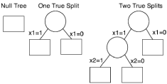
    Figure 1:  Simulated Tree Structures. The following tree structures were
simulated to test our adjusted prognostic and adjusted interaction tree
algorithms.
Extended simulations with 40% censoring, 60% censoring, 2:1 unbalanced treatment, weak correlation between the associated SNP and the confounder, and strong correlation between the associated SNP and confounder were performed. For each of these simulations the default parameter values defined above were used.
Results
The model performance under the ‘null’ is shown in Table 1 and Table 2. The model performs well with only a 1.4% to 8.4% chance of selecting the wrong tree, and with no obvious trends when varying any parameters. Note that although in the selection of the final tree we penalize each split by 4, which roughly correspond to the 0.05 confidence level for a Χ² random variable, this does not imply an expected 5% chance of selecting the wrong tree under the null.
![]()
    Splitting Rule
    Sample    Size(n)


    1000
    900
    800
    700
    600
    400
    300
    200


    Ga
    .029
    .045
    .051
    .048
    .061
    .049
    .064
    .054


    Gi
    .049
    .068
    .054
    .042
    .047
    .038
    .032
    .014


    Gai
    .071
    .070
    .051
    .069
    .059
    .047
    .045
    .022
Table 1: Tree performance under the null hypothesis given different sample size.
![]()
    Splitting Rule
    Number of    Potential Splits


    1000
    500
    250
    100
    50
    10


    Ga
    .084
    .057
    .055
    .038
    .032
    .024


    Gi
    .044
    .054
    .051
    .048
    .047
    .035


    Gai
    .039
    .053
    .058
    .040
    .058
    .058
Table 2: Tree performance under the null hypothesis given different number of
potential splits.
Under the ‘alternative’ we first consider the probability that the true tree is identified as an optimally pruned sub tree by the pruning algorithm in section 2.3. If this does not occur, then our method to choose the final tree out lined in section 2.4 will automatically fail. Of the times that the true tree is identified as an optimal sub tree, we then calculate the probability that the final tree we select with our resampling method is the correct one. Recall that the structure of the true tree is shown in Figure1.
For the prognostic tree, Figure 2 shows the probability of selecting the true tree when it has two splits and Figure 3 shows the power when the true tree has one split. Figure 4 and 5 show the probability of identifying the true tree as an optimal sub tree when the true tree has two and one splits respectively. Figures 6, 7, 8, and 9 show the results for the interaction tree. The effect of modifying our simulation parameters is very similar across all splits, probabilities, and true tree structures.
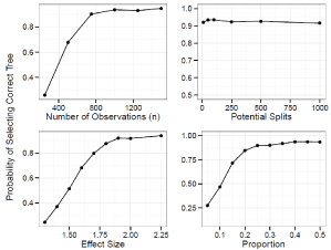
    Figure 2:  Simulation Results: Adjusted Prognostic Tree, Two True Splits.
The probability of our adjusted prognostic tree algorithm selecting the true
tree as the final tree.
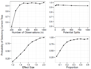
    Figure 3:  Simulation Results: Adjusted Prognostic Tree, One True Split. The
probability of our adjusted prognostic tree algorithm selecting the true tree
as the final tree.
In general the power to identify and select the correct tree increase as n (and the underlying number of events) increases, the effect size increases, and the split becomes more balanced. Although the power decrease as the number of potential splits increases, this decrease is relatively small, and it is quite robust to the high dimension of the covariate space. The power to identify the true tree as an optimal sub tree is usually quite high. See Figure 4, 5, 8 and 9 for more detail.
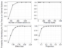
    Figure 4:  Simulation Results: Adjusted Prognostic Tree, Two True Splits. The
probability of our adjusted prognostic tree algorithm selecting the true tree as
an optimal sub tree.
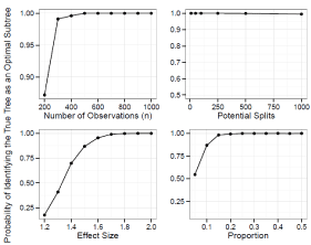
    Figure 5:  Simulation Results: Adjusted Prognostic Tree, One True Split. The
probability of our adjusted prognostic tree algorithm selecting the true tree as
an optimal sub tree.
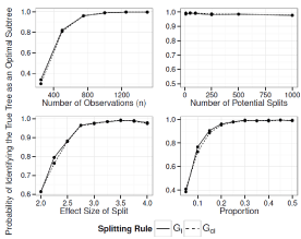
    Figure 6:  Simulation Results: Adjusted Interaction Tree, Two True Splits. The
probability of our adjusted iteration tree algorithm selecting the true tree as
the final tree.
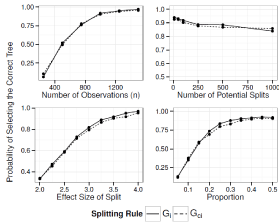
    Figure 7:  Simulation Results: Adjusted Interaction Tree, One True Split. The
probability of our adjusted iteration tree algorithm selecting the true tree as
the final tree.
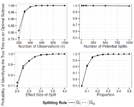
    Figure 8:  Simulation Results: Adjusted Interaction Tree, Two True Splits. The
probability of our adjusted interaction tree algorithm selecting the true tree as
an optimal sub tree.
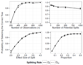
    Figure 9:  Simulation Results: Adjusted Interaction Tree, One True Split. The
probability of our adjusted interaction tree algorithm selecting the true tree as
an optimal sub tree.
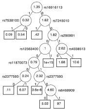
    Figure 10:  Real data adjusted interaction tree. The final tree selected by our
pruning algorithm. The hazard ratio of treatment for each subgroup is written
inside each node. The name of the SNP being split is written beside each
node. The labels1 and 0 are an indicator of having at least one copy of them
in oral lele in the respective SNP.
Table 3 and 4 show that the power to choose the correct tree decreases when the censoring increases to 40% and 60%. Unbalanced 2:1 treatment, weak correlation between the associated SNP and the confounder, and strong correlation between the associated SNP and the confounder have relatively little impact on the power to choose the correct tree. The power to identify the correct tree as an optimal sub tree remains high even with 40% and 60% censoring.
![]()
    G
    # Splits
    Standard
    60% Censor
    40% Censor
    2:1 treat
    Strong Corr
    Weak Corr


    Gai
    2
    0.90
    0.43
    0.75
    0.84
    0.89
    0.92


    Gai
    1
    0.92
    0.56
    0.84
    0.89
    0.92
    0.93


    Gi
    2
    0.92
    0.46
    0.75
    0.84


    Gi
    1
    0.96
    0.56
    0.83
    0.90


    Ga
    2
    0.93
    0.56
    0.83

    0.87
    0.94


    Ga
    1
    0.95
    0.73
    0.91

    0.90
    0.94
Table 3: Tree performance under extended simulation settings. For each of the
three simulated splitting rules Gai, Gi, and Ga and with true tree structures of 1
and 2 splits, the probability that the pruning algorithm picks the true tree as an
optimal sub tree is shown. The result from the standard simulation is compared
with simulations with 60% censoring, 40% censoring, 2:1 unbalanced treatment,
strong correlation between the associated SNP and the confounder and
weak correlation between the associated SNP and the confounder. Extended
simulation settings not relevant to a particular splitting rule are omitted.
![]()
    G
    # Splits
    Standard
    60% Censor
    40% Censor
    2:1 treat
    Strong Corr
    Weak Corr


    Gai
    2
    0.993
    0.705
    0.971
    0.988
    0.996
    0.990


    Gai
    1
    1.000
    0.895
    0.988
    0.997
    0.998
    1.000


    Gi
    2
    0.990
    0.728
    0.970
    0.982


    Gi
    1
    1.000
    0.932
    0.987
    0.999


    Ga
    2
    0.999
    0.869
    0.982

    0.996
    0.999


    Ga
    1
    1.000
    0.966
    0.998

    0.996
    1.000
Table 4: Tree performance under extended simulation settings. For each of the
three simulated splitting rules Gai, Gi, and Ga and with true tree structures of 1
and 2 splits, the probability that the pruning algorithm picks the true tree as the
final sub tree is shown. The result from the standard simulation is compared
with simulations with 60% censoring, 40% censoring, 2:1 unbalanced treatment,
strong correlation between the associated SNP and the confounder and
weak correlation between the associated SNP and the confounder. Extended
simulation settings not relevant to a particular splitting rule are omitted.
Prognostic tree results
When the true tree has two splits the power to select the correct tree decreases sharply when n<750, going from 90% at 750 down to 68% at 500, and 26% at
250. The power stays around 94% from 1000 to 1500. Modifying the balance of the split has a similar effect, with the power decreasing sharply when the balance is less than 1:4, going from 85% at 1:4, down to 69% at 1:57, 47% at 1:9 and 27% at 1:19. As the split becomes more balanced than 1:4 the power increases steadily until it reaches 93% when balanced. The power increases linearly from 24% to 88% as the effect size has increased from 1.3 to 1.8. The power goes to 92% at 1.9 and reaches 94% at 2.25. The power is quite robust to the number of potential splits, going from 92% at 10 potential splits, to 90% at 100, 87% at 500, and 86% at 1000.
When the true tree has one split the power to select the correct tree decreases sharply when n<400, going from 91% at 400 down to 91% at 300, and 52% at 400. The power increases to 9% at 500 and stays relatively flat until 1000. Varying the balance of the split has a similar effect. The power decreases sharply when the balance is less than 1:3 going from 92% at 1:3 down to 83% at 1:4, 70% at 1:57, 50% at 1:9 and 29% at 1:19. The power reaches 94% at 1:1.86, and reaches 95% when balanced. The power increases linearly from 16% to 81% as the effect size is increased from 1.2 to 1.7. The power goes to 87% at 1.8, 93% at 1.9 and 95% at 2. The power is extremely robust to the number of potential splits, staying around 94% from 10 to1000.
Interaction tree results
When the true tree has two splits the power to select the correct tree decreases sharply when n<1000, going from 90% at 1000 down to 78% at 750, 50% at 500, and 11% at 250. The power increases to 94% at 1250 and reaches 95% at 1500. Modifying the balance of the split has a similar effect, with the power decreasing sharply when the balance is less than 1:4, going from 80% at 1:4, down to 69% at 1:57, 38% at 1:9 and 12% at 1:19. As the split becomes more balanced than 1:4 the power increases steadily until it reaches 89% at 1:1.5, and finally reaches 90% at 1:1. The power increases linearly from 34% to 71% as the effect size is increased from 2 to 2.75. The power goes to 79% at 3, 90% at 3.5 and 95% at 4. The power is extremely robust to the number of potential splits, staying around 92% from 10 to 1000.
When the true tree has one split the power to select the correct tree decreases sharply when n<500, going from 92% at 500 down to 83% at 400, 69% at 300, and 40% at 200. The power increases to 96% at 600 stays fairly stable, increasing to 97% at 1000. Varying the balance of the split has a similar effect. The power decreases sharply when the balance is less than 1:4, going from 78% at 1:4, down to 61% at 1:57, 40% at 1:9 and 16% at 1:19. Increasing the balance past 1:4 raises the power steadily until it reaches 92% at 1:2.5. The power is then stable until it is balanced. The power increases linearly from 37% to 76% as the effect size is increased from 2 to 2.75. The power goes to 83% at 3, 92% at 3.5 and 96% at 4. The power is quite robust to the number of potential splits, going from 94% at 10 potential splits, to 92% at 100 and 89% at1000.
Application to randomized clinical trial
Head and neck Cancer (HNC) is the 5th most common type of cancer world-wide, with 650,000 new cases per year [17]. Most patients present with locally-advanced disease, with 5 year Overall Survival (OS) rates of about 50%, which have not improved over the decades [18]. The use of antioxidant vitamins to supplement chemo and radiation therapy in cancer patients has had conflicting results. Some studies have shown that this regime leads to better survival outcomes, while others have shown that it leads to worse [19]. It is possible that this conflicting evidence could be driven by complex gene-treatment interactions. To explore such genetic hypotheses one must take care to control for population stratification, which is a major source of spurious results in genetic studies defined as the difference in allele frequencies in patients stemming from their ancestral differences [20]. The standard way to control for population stratification is to adjust for the main principal components of the ancestral differences [21]. Therefore we will use our adjusted interaction survival tree method to find subgroups of patients that respond most differently to antioxidant vitamins based on their genetic signature, while adjusting for the main principal components of their ancestral differences.
We analyzed the recurrence free survival of 540 patients with HNC from a randomized a-tocopherol/β-carotene placebocontrolled Genome Wide Association Study (GWAS) with 620,901 Single-Nucleotide Polymorphism (SNPs) [22]. After standard genetic quality control procedures, 515 patients, 261 randomized to the treatment arm and 254 randomized to a placebo provided genotype information for 543,873 SNPs. We calculated the principal components of the ancestral differences of the patients, and adjusted our tree by the top three. We built a tree with 10 splits from the 100 most prognostically significant SNPs. The dominant model was used for each SNP, transforming the SNP variable to an indicator of having at least one minor allele. We pruned the tree with 1,000 boot strap samples and penalized each split by two. The final tree can be seen in Figure 10. Inside each node is the hazard ratio of treatment. A hazard ratio greater than 1 indicates that taking the antioxidant vitamin leads to a worse outcome than taking the placebo, while a hazard ratio less than 1 indicates that taking the vitamin leads to a better outcome. Although this is the best tree according to the automated pruning process, the tree can be further pruned by domain experts to remove statistically significant but clinically insignificant splits. Our method can identify subgroups of patients with specific genetic signatures for which the treatment has high efficacy.
Discussion and Conclusion
The novel methods we have introduced can help translational research in genetic studies and personalized medicine. Scientists can use our methods to control for confounders when identifying complex GxG and GxE interactions or identifying the best treatment choice for patients based on their genetic profile. Moreover we have shown that the interaction survival tree can perform well with the large number of genetic factors often found in personalized medicine research. Once a tree is created and subgroups are identified, summary statistics such as hazard ratios of treatment, Kaplan-Meier curves [23], and median survival times for each group can be presented to clinicians. They can then use t statistics, in combination with their clinical consideration to classify the prognosis or select the best treatment to their patients while controlling for potential confounders. Simulations have shown that the probability of selecting the wrong tree under the null hypothesis has been well controlled (at only 1.4-8.4%) and that the power of selecting the true tree under the alternative hypothesis is usually high. To have adequate power there should be a sufficiently large number of events and interactive effect between the split and treatment. One must be particularly aware of the balance of the potential splits as power decreases dramatically for splits with balance worse than1:4. Therefore, these methods will likely be under powered when used for genetic markers (i.e. SNPs) with low minor allele frequency. If these criteria are met, then our method is very robust to the number of potential splits, with the power being stable with a large number of covariates (up to 1000 in the simulations). Using a more efficient implementation of the algorithm and parallel computing, models with an even larger number of potential splits should also perform well.
In addition to being scientifically relevant, adjusting for confounders in the splitting rule seems to have statistical benefits. Our simulations have shown that adjusting for a confounder is much more efficient than creating a new split. Indeed, we needed to double our sample size from 500 to 1000 to have similar power when the true tree structure changed from one to two splits, however controlling for 4 confounders only resulted in a slight drop in power. Further research into splitting rules that move more of the modelling into the splits themselves rather than the topology of the tree seems worth pursuing.
In the pruning algorithm the cross-validated goodness of split is calculated as the mean of the goodness-of-split of trees built from a single fold of data.
One must be especially careful about the number of folds, f, since the sample size |Lj|≈n/f used to make the tree Tj,k must be large enough to support the true tree structure. The number of folds can then be seen as a sparsity parameter with more folds resulting in sparser trees. Similar consideration must also be taken when choosing the number of confounding variables to include in the model. When working with such small sample sizes, along with the usual concerns about the instability of asymptotic results, the vector corresponding to the splits may be deemed computationally singular with the confounding variables, leading to G(s, h) = 0 and sparser trees.
When selecting the final tree choosing the penalty parameter αc=4 corresponds to the 0.05 significance level of a Χ² random variable which is approximately 4. This choice is reasonable when treatment has only two levels, because the ‘honest’ LRT statistic of the split will be asymptotically Χ². In general, when we have k levels of treatment the ‘honest’ LRT statistic of the split will be asymptotically Χ² and the choice ofαccould be chosen as the 0.05 significance level of a Χ² random variable.
In addition to the LRT statistic, we also tested using other novel splitting methods such as the Wald test statistic and absolute value of the fitted parameter of an underlying Cox model. All three splitting rules were found to have similar performance, and the LRT statistic was chosen as it is the most generalizable. Indeed the recursive partitioning algorithm we use is not dependent on the particular choice of model, and other likelihood based models could be used. With some slight modifications the idea of splitting by the ratio of two likelihoods could be extended to any situation in which a likelihood space can be defined.
The current adjusted survival tree models are developed based on the Cox models. However, for the real research studies, some time to event outcomes may not fit the proportional hazard assumption. We suggest applying proportional hazard assumption test on the data before applying the survival tree model. Further extensions of the adjusted survival tree model are in development to deal with other types of time to event outcomes.
Author’s Contributions
WX and RD Bareco-first authors and are equal contributors to the development and implementation of the adjusted survival tree methodology. IB, FM, and GL provided data for the application of the methodology to the randomized clinical trial.
Acknowledgement
The authors would like to thank the COMBIEL training program for supporting this study, and RDB thanks the High Impact Clinical Trial program of the Ontario Institute of Cancer Research for his generous funding.
References
- James N Morgan and John A Sonquist. Problems in the analysis of survey data, and a proposal. Journal of the American Statistical Association. 1963; 58: 415-434.
- Leo Breiman, Jerome H Friedman, Richard A Olshen, Charles J Stone. Classification and regression trees. Wads worth & brooks. Monterey, CA. 1984.
- Steffens M, Lamina C, Illig T, Bettecken T, Vogler R, Entz P, et al. SNP-based analysis of genetic substructure in the German population. Hum Hered. 2006; 62: 20-29.
- Hennis AJ, Hambleton IR, Wu SY, Leske MC, Nemesure B. Barbados National Cancer Study Group. Breast cancer incidence and mortality in a Caribbean population: comparisons with African-Americans. Int J Cancer. 2009; 124: 429-433.
- Su X, Fan J. Multivariate survival trees: a maximum likelihood approach based on frailty models. Biometrics. 2004; 60: 93-99.
- Hemant Ishwaran, Udaya B Kogalur, Eugene H Blackstone, Michael S Lauer. Random survival forests. The Annals of Applied Statistics. 2008; 841-860.
- Su X, Zhou T, Yan X, Fan J, Yang S. Interaction trees with censored survival data. Int J Biostat. 2008; 4: Article 2.
- Sevin BU, Lu Y, Bloch DA, Nadji M, Koechli OR, Averette HE. Surgically defined prognostic parameters in patients with early cervical carcinoma. A multivariate survival tree analysis. Cancer. 1996; 78: 1438-1446.
- Chen J, Yu K, Hsing A, Therneau TM. A partially linear tree-based regression model for assessing complex joint gene-gene and gene-environment effects. Genet Epidemiol. 2007; 31: 238-251.
- Evans WE, Relling MV. Moving towards individualized medicine with pharmacogenomics. Nature. 2004; 429: 464-468.
- Aspinall MG, Hamermesh RG. Realizing the promise of personalized medicine. Harv Bus Rev. 2007; 85: 108-117, 165.
- Lesko LJ. Personalized medicine: elusive dream or imminent reality? Clin Pharmacol Ther. 2007; 81: 807-816.
- Hamburg MA, Collins FS. The path to personalized medicine. New England Journal of Medicine. 2010; 363: 301-304.
- Yusuf S, Wittes J, Probstfield J, Tyroler HA. Analysis and interpretation of treatment effects in subgroups of patients in randomized clinical trials. JAMA: the journal of the American Medical Association. 1991; 266: 93-98.
- Harrell FE, Lee KL, Mark DB. Multivariable prognostic models: issues in developing models, evaluating assumptions and adequacy, and measuring and reducing errors. Stat Med. 1996; 15: 361-387.
- Leblanc M, Crowley J. Survival trees by goodness of split. Journal of the American Statistical Association. 1993; 88: 457-467.
- Jemal A. Global burden of cancer: opportunities for prevention. Lancet. 2012; 380: 1797-1799.
- Pfister DG, Ang KK, Brizel DM, Burtness BA, Cmelak AJ, Colevas AD, et al. Head and neck cancers. J Natl Compr Canc Netw. 2011; 9: 596-650.
- Lawenda BD, Kelly KM, Ladas EJ, Sagar SM, Vickers A, Blumberg JB. Should supplemental antioxidant administration be avoided during chemotherapy and radiation therapy? J Natl Cancer Inst. 2008; 100: 773-783.
- Cardon LR, Palmer LJ. Population stratification and spurious allelic association. Lancet. 2003; 361: 598-604.
- Price AL, Patterson NJ, Plenge RM, Weinblatt ME, Shadick NA, Reich D. Principal components analysis corrects for stratification in genome-wide association studies. Nat Genet. 2006; 38: 904-909.
- Bairati I, Meyer F, Jobin E, Gélinas M, Fortin A, Nabid A, et al. Antioxidant vitamins supplementation and mortality: a randomized trial in head and neck cancer patients. Int J Cancer. 2006; 119: 2221-2224.
- Kaplan EL, Meier P. Non parametric estimation from in-complete observations. Journal of the American statistical association. 1958; 53: 457-481.