
Research Article
Austin J Biotechnol Bioeng. 2015;2(1): 1036.
Development of a Simple Kinetic Model and Parameter Estimation for Biomass and Nattokinase Production by Bacillus subtilis 1A752
Rajasekar Vinayagam1*, Ramachandra Murty Vytla1 and Muthukumaran Chandrasekaran2
1Department of Biotechnology, Manipal Institute of Technology, Manipal, India
2Department of Industrial Biotechnology, Government College of Technology, Coimbatore, India
*Corresponding author: Rajasekar Vinayagam, Department of Industrial Biotechnology, Government College of Technology, Coimbatore-641013, Tamilnadu, India.
Received: December 16, 2014; Accepted: February 25, 2015; Published: February 27, 2015
Abstract
Nattokinase is a novel promising thrombolytic agent. Nattokinase fermentation by Bacillus subtilis 1A752 was modeled using unstructured kinetic models to depict the importance of growth and growth associated production. The logistic and Luedeking–Piret equations were used in batch fermentation with regard to glucose utilization and time. Model parameters (X0, μm, m, n, p and q) were determined by non linear regression using Matlab and the predicted parameter values had good agreement with the experimental data. Excellent significant R2 values of 0.998, 0.924 and 0.998 were observed for biomass, nattokinase production and substrate utilization. A simulink model was developed by considering the parameter values obtained from the ?tting of batch culture data which can be a useful tool for scaling up the nattokinase production with consistency.
Keywords: Nattokinase; Growth kinetics; Production kinetics; Kinetic parameters; Fermentation; Matlab
Abbreviations
t-PA: Tissue Plasminogen Activator inhibitor; TCA: Trichloroactetic Acid; t: Fermentation time (h); X: Cell concentration, gL-1; X0: Initial cell concentration gL-1; Xm: Maximum cell concentration gL-1; Xpre: Predicted cell concentration gL-1; P: Nattokinase activity 1 μmol of tyrosine released per min; P0: Initial product concentration (μ/mL); Ppre: Predicted product concentration (μ/mL); S: Glucose gL-1; S0: Initial substrate concentration gL-1; Spre: Predicted substrate concentration gL-1; YX/S: Yield factor for cells on glucose substrate (gbiomass -1 gglucose -1): RMSE: Root Mean Square Error; μm: Maximum specific growth rate (h-1); m: Growthassociated product formation coefficient (U gbiomass -1); n: Non-growthassociated product formation coefficient (U gbiomass -1 h-1); p: Substrate utilization rate constant (gbiomass -1 gglucose -1); q: Maintenance coefficient (gglucose gbiomass h-1)
Introduction
Nattokinase (E.C 3.4.21.62) is an effective fibrinolytic enzyme which belongs to serine alkaline protease family. It was originally isolated from Japanese traditional food ‘natto’ by Sumi H et al. [1]. This enzyme possesses plasminogen activator activity by cleaving the tissue plasminogen activator (t-PA) inhibitor type I which leads to lysis of blood clot in the Human system and it is also able to digest fibrin directly by proteolysis [2,3]. Fibrinolytic activity of nattokinase is reported to have four times higher activity than plasmin [4]. Nattokinase can be used as a potent drug for thrombosis therapy as it has stronger fibrinolytic activity than other commercial drugs [5].
The bioprocess which involves microbial cells is complex in nature and is a critical step for better operation to achieve maximum product output [6]. Behavior of the microbial system can be evaluated by the development of kinetic models and experimental designs,which solves the design and control of bioprocess problems [7,8]. Structured and unstructured models are generally used to express the microbial processes [9]. Structured model is a complex in which the biomass is divided into compartments; cell structure and composition which are considered for developing the model. Biological system can be clearly elucidated by unstructured model considering the biomass and product formation alone. In this study, unstructured models for microbial growth (Logistic model) and product formation (Luedeking-Piret model) are considered in order to evaluate the batch fermentation process.
Nattokinase production is carried out by fermentation using Bacillus strains [10,11]. Recent research on nattokinase is mainly focused on screening of microorganisms, optimization, purification studies and only limited work has been made for kinetic modeling of nattokinase production [12,13]. The knowledge about the process kinetics for nattokinase production is of great impact on the economics in large scale operations. Till date, few reports were available in the literature on the development of a simple kinetic model in order to investigate the correlation among growth, production formation and substrate utilization for nattokinase production [6].
The present study is focused on the development of a simple kinetic model for nattokinase production by using experimental data obtained from batch bacterial fermentation in shake flask culture under optimum conditions. The relation of nattokinase production with biomass and the effect of substrate were studied by using the mathematical models. Kinetic parameter values of mathematical model were estimated by Matlab and the Simulink model was developed to understand the nattokinase fermentation kinetics.
Materials and Methods
Microorganism and chemicals
Bacillus subtilis 1A752 strain was procured from Bacillus Genetic Stock Center, USA as a gift sample for present work. For routine work the bacteria was maintained on nutrient agar slants. The slants were kept at 4°C and sub-cultured every 20 days. All the chemicals used in this study were analytical grade and procured from Hi-media, India.
Fermentation conditions
Five percent of inoculum culture was added to Erlenmeyer flasks (250 mL) containing 45 mL optimized production media composed of in percentage: Glucose - 1.0; Peptone - 3.0; MgSO4 - 0.2 and CaCl2 - 0.5. The pH of the medium was adjusted to 7.0. The flasks were incubated at 37°C for 24 hr and the samples were drawn at 2 hr interval for biomass and enzyme activity determination.
Biomass estimation
Bacterial growth was estimated by measuring the optical density of the fermentation broth at 600 nm and was converted to cell dry weight (gL-1) based on the biomass versus cell dry weight standard. The culture was centrifuged at 5000 x g at 4°C for 10 min and the clear cell-free supernatant was used for the measurement of glucose concentration and nattokinase activity.
Nattokinase activity assay
Nattokinase activity was determined using fibrin as a substrate by modifying the method reported by Liu J et al. [14]. Enzyme solution (0.5 mL) was suitably diluted and was mixed with 1 mL of 1% fibrin in 0.2M NaOH (pH 7.8). This reaction was allowed for 10 min at 37°C in water bath for 15 min before the assay. Then the mixture was kept undisturbed at room temperature for few min. Digested fibrin was precipitated by adding the Trichloroactetic Acid (TCA). The mixture was then centrifuged at 5000 rpm for 3 min; the filtrate was collected and added to 5 mL of 0.5 M sodium carbonate. The optical density was measured at 280 nm and nattokinase activity was calculated by using the tyrosine standard. One unit of nattokinase activity is defined as the amount of enzyme required to release 1 μmol of tyrosine per min at standard assay conditions.
Residual sugar estimation
Glucose content in the fermentation broth was estimated using the Dinitrosalicylic Acid (DNS) method [15]. Briefly, 0.5 mL of cell-free broth was diluted to 2.5 mL with distilled water and mixed thoroughly with 3 mL of DNS. The mixture was then boiled for 5 min and diluted sufficiently to 10 mL with distilled water. The final solution was used to measure the absorbance at 540 nm using a UV–visible spectrophotometer, and the glucose concentration was calculated using glucose standard curve.
Kinetic model
The modeling of rate equations for biomass (X), nattokinase activity (P) and glucose (S) were used to explain the fermentation process.
Microbial growth kinetics
The unstructured models which were widely used to describe the microbial cell growth are the Monod model and logistic equation. Characterization of cell growth in several microbial fermentation processes is well studied using the logistic equation which is a substrate independent model [16,17].
The growth pattern of logistic kinetics can be described as follows:
(1)
Where X is biomass concentration (gL-1), Xm is the maximum biomass concentration (gL-1), μm is the maximum specific growth rate (h-1) and t is the time (h). The integration of Eq. (1) yields Eq. (2) with the initial conditions of X = X0 at t = 0:
(2)
Rearranging the Eq. (2) gives Eq. (3)
(3)
The value of μm and X0 can be obtained from the slope and y-intercept of the plot between and time (t). The value of Xm is determined from the experimental data.
Product formation kinetics
Nattokinase production kinetics was studied using Luedeking- Piret model [18]. This model explains that the product formation rate is related linearly with biomass concentration (X) and the growth rate (dX/dt).
(4)
Where m and n are the kinetic constants for product formation. The value of ‘n’ can be obtained from the stationary phase data of microbial growth at which it is assumed that (dX/dt = 0) and (X = Xm) and the following expression is used to determine ‘n ‘value.
(5)
Eq. (4) is rearranged as follows to express P as a function of time (t)
dP = m dX + n ∫ X(t)dt (6)
The product formation rate equation (Eq.7) can be arrived by integrating Eq. (4) using Eq. (2) with the initial conditions P = 0 at t = 0:
(7)
Eq. (7) is written in the following simple form:
P = m a(t) + n β(t) (8)
Where
(9)
(10)
The growth associated product formation rate constant ‘m’ can be determined by plotting a graph (P – n β(t)) versus a(t) and non growth associated product formation rate constant ‘n’ can be determined by using Eq. (5).
Substrate utilization kinetics
Glucose is used as a limiting substrate for nattokinase production which acts as carbon source for both biomass growth and product synthesis. The substrate utilization kinetics is usually represented by the following equation.
Where p = 1/YX/S and q is maintenance coefficient (ms). These two parameters (p and q) can be determined by the same procedure followed for product formation kinetics. Maintenance coefficient can be estimated by the following equation at stationary phase (dX/dt = 0; X = Xm).
(12)
Eq. (11) is rearranged as follows to evaluate ‘p’
-dS = p dX + q ∫ X(t)dt (13)
Substituting Eq. (2) in Eq. (13) and integrating with initial conditions (S = S0; t = 0) gives the following equation:
(14)
Eq.14 is rewritten in the following form to evaluate ‘p’
S = S0 – p γ(t) – q δ(t) (15)
Where
(16)
The value of ‘p’ can be determined from the slope of the plot between (S0 – S – q δ(t)) and γ(t).
Model parameters estimation
Kinetic models which describe the microbial process on a particular substrate are nonlinear which in turn makes parameter estimation relatively difficult. Though few models can be linearized, their utilization is limited because of the error associated with the transformation of dependent variable and therefore resulted in inaccurate parameter estimations. Hence, the nonlinear least-squares regression is often used to estimate kinetic parameters from nonlinear expressions. The parameter estimates obtained from the linearized kinetics expressions can be used as initial estimates in the iterative nonlinear least-squares regression using the least square curve fit in order to fit the developed models and to estimate the parameters (substrate consumption, biomass and product formation). The error between observed and predicted values was minimized by adjusting the number of iterations in the system. MATLAB command ‘lsqcurvefit’ was used to estimate and evaluate the significance of the parameters by fitting the experimental values to the proposed mathematical models. Each experiment was repeated twice and the results were reported as averaged values. To evaluate accuracy of the kinetic models, statistical parameters such as root mean square error and correlation regression coefficient were used [6].
(18)
Where, X, X´ and Xav are experimental, predicted and average values of biomass (X), product (P) and substrate (S) respectively.
Results and Discussions
Microbial growth
Nattokinase fermentation by B. subtilis 1A752 shows the conventional growth pattern in batch process using glucose based synthetic medium. Logistic equation (Eq. 3) is used to fit the batch fermentation growth kinetics data. A significant increase in nattokinase production is observed from 4th hour of fermentation and reached maximum at 12th hour and decreased gradually. Time required for achieving maximum enzyme production is much lesser (50 %) compared to the previous report [6]. Maximum biomass (2.8gL-1) was obtained at 22nd h of fermentation and remains constant due to depletion of glucose in the medium. By using Xm = 2.8 gL-1 from the experimental data in Eq. (3), μm and X0 were determined as 0.364 h-1 and 0.199 gL-1 respectively from slope and intercept of (Figure 1). X0 value of experimental and calculated were found similar in this study. The proposed logistic model was adequate to explain the sigmoidal profile of bacterial growth as reported earlier [9,19,20].
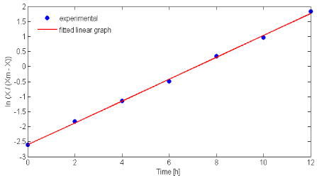
    Figure 1:  Estimation of maximum specific growth rate (μm) and initial
substrate concentration (X0) using Eq. (3).
Product formation
Nattokinase production followed Luedeking- Piret model and the kinetic parameters were evaluated by using Eq. (8) at stationary phase (dX/dt = 0). The growth associated rate constant ‘m’ and non-growth associated rate constant ‘n’ were obtained from (Figure 2) as 388.52 Ugbiomass -1 and -3.59 Ugbiomass -1h-1 respectively. These results showed that the degree of growth associated constant ‘m’ is much greater than the non-growth associated rate constant ‘n’. Hence, the nattokinase production in this study was observed as growth associated product formation and it had good agreement with alkaline protease production by Bacillus circulans reported by Subba Rao C et al. [21]. On the other hand, Mahajan PM et al. [6]. has stated that nattokinase production was observed as non-growth associated product using Bacillus natto [6]. The reasons for variations in the results may be due to the microorganisms used and the environmental conditions for nattaokinase production.
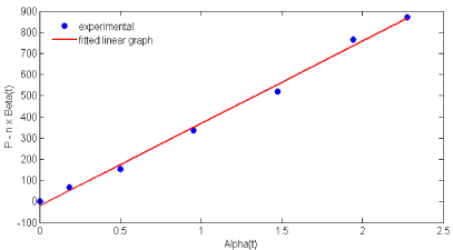
    Figure 2:  Estimation of non- growth associated (m) and growth associated
(n) parameters using Eq. (8).
Substrate utilization
In nattokinase fermentation, biomass concentration was increased with the decrease in the glucose level in the medium. Glucose consumption was gradually reduced from the commencement of the fermentation and maximum depletion was observed at 24 h. Glucose utilization kinetics was represented in Eq. (15) and the initial glucose concentration used in this study was 10gL-1. A plot of Eq. (15) shown in (Figure 3), yielded p = 2.313 gbiomass g substrate -1 and q= 0.14 gglucose gbiomass -1 h-1 from slope and the intercept. Maintenance coefficient (ms) was used to explain the specific uptake rate of substrate for cellular maintenance and it was found to be varied with initial substrate concentrations. Sinclair CG et al. [22] reported the range of ms values as low from 0.02 to 4.0 gsubstrate gbiomass -1 h-1 and our obtained ms value was within the reported range [22].
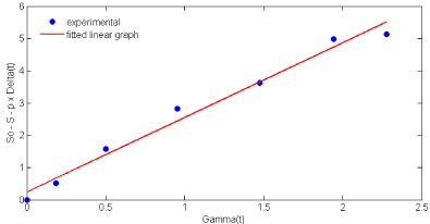
    Figure 3:  Estimation of substrate utilization kinetic parameters (p and q)
using Eq. (15).
Model testing
Matlab 2011b was used to estimate the kinetic parameters (μm, X0, Xm, m, n, p, q, Yx/s, Yp/s) by using ‘lsqcurvefit’ function. The estimated parameters were used to test the model. A comparison of experimental and simulated data for X, P and S was shown in (Figure 4). Experimentally calculated and simulated parameter values were summarized in Table 1. R2 value is generally used to describe the goodness of fit for the experimental and predicted data. In this study, R2 values for biomass, nattokinase activity and substrate utilization were found to be 0.99, 0.92 and 0.99 respectively. These R2 values confirmed that the proposed model provide the better predictions. A Simulink model was developed to represent biomass, nattokinase activity and substrate utilization and the estimated parameter values were used to simulate the model (Figure 5). The output of the Simulink model is in accordance with the experimental results.
Model Parameters
Experimental
Predicted
X0 (gL-1)
0.199
0.188
Xm (gL-1)
2.88
2.880
�m (h-1)
0.364
0.374
m ( U gbiomass-1)
388.52
293.82
n (U gbiomass-1 h-1)
-3.593
0
p (gbiomass gglucose-1 )
2.313
3.066
q (gglucose gbiomass-1 h-1)
0.14
0.5
Table 1:  Estimated experimental and predicted kinetic model parameter values
for Nattokinase production by Bacillus subtilis 1A752.
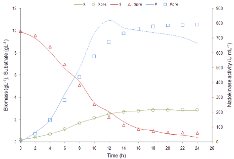
    Figure 4:  Comparison of time course profile for experimental (−−−) and
predicted data (open symbols) of biomass, nattokinase production and
substrate utilization respectively in batch fermentation.
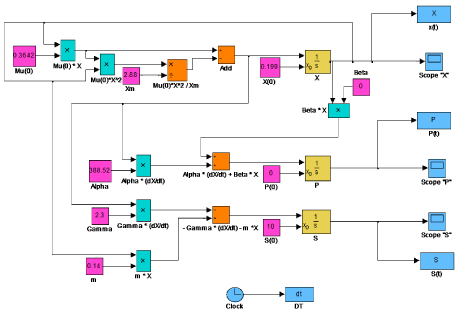
    Figure 5:  Developed Simulink model for nattokinase production for evaluation
of biomass (X), nattokinase production (P) and substrate utilization (S) in
batch fermentation.
Conclusion
Microbial fermentation is complex and it is quite difficult to understand the complete details of the process. The model proposed in this study describes the biomass, nattokinase production and substrate utilization with culture time in a good manner. Growth pattern follows the logistic model and the parameters were determined and experimental determination of Xm was the major limitation of this model. Nattokinase production was represented by Luedeking-Piret model and based on the estimated kinetic parameter values, it was noticed that nattokinase production by Bacillus subtilis 1A752 was growth associated. High significance of correlation (R2) was observed with the experimental and predicted results. In view of the above, the developed model may be useful for controlling the growth, nattokinase production and substrate consumption kinetics in large scale fermentation using Bacillus subtilis 1A752.
Acknowledgement
The first author gratefully acknowledges the Department of Biotechnology, MIT, Manipal University, for providing the facilities to carry out the research work.
References
- Sumi H, Hamada H, Tsushima H, Mihara H, Muraki H. A novel ?brinolytic enzyme (nattokinase) in the vegetable cheese Natto; a typical and popular soybean food in the Japanese diet. Experientia. 1987; 43: 1110-1111.
- Fujita M, Hong K, Ito Y. Thrombolytic effect of Nattokinase on a chemically induced thrombosis model in rat. Biol Pharm Bull. 1995; 18: 1387-1391.
- Chang CT, Fan MH, Kuo FC, Sung HY. Potent ?brinolytic enzyme from a mutant of Bacillus subtilis IMR-NK1. J Agric Food Chem. 2000; 48: 3210-3216.
- Sumi H, Nakajima N, Mihara H. In vitro and in vivo ?brinolytic properties of nattokinase. Thromb. Haemost. 1992; 89: 1267.
- Peng Y, Yang X, Zhang Y. Microbial ?brinolytic enzymes: An overview of source, production, properties, and thrombolytic activity in vivo. Appl. Microbiol Biotechnol. 2005; 69: 126-132.
- Mahajan PM, Gokhale SV, Lele SS. Production of nattokinase using Bacillus natto NRRL 3666: Media optimization, scale up, and kinetic modeling. Food. Sci. Biotechnol. 2010; 19: 1593-1603.
- Voll F, Krüger RL, Castilhos FD, Filho LC, Cabral V, Ninow J, et al. Kinetic modeling of lipase-catalyzed glycerolysis of olive oil. Biochem. Eng. 2011; 56: 107-115.
- Xu LJ, Liu YS, Zhou LG, Wu JY. Modeling of Fusarium redolens Dzf2 mycelial growth kinetics and optimal fed-batch fermentation for beauvericin production. J. Ind. Microbiol. Biotechnol. 2011; 38: 1187-1192.
- Murat E, Ferda M. A kinetic model for actinorhodin production by Streptomyces coelicolor A3(2). Process. Biochem. 1999; 34: 625-631.
- Kwon EY, Kim KM, Kim MK, Lee IY, Kim BS. Production of nattokinase by high cell density fed-batch culture of Bacillus subtilis. Bioprocess. Biosys. Eng. 2011; 34: 789-793.
- Dabbagh F, Negahdaripour M, Berenjian A, Behfar A, Mohammadi F, Zamani M, et al. Nattokinase: production and application. Appl. Microbial. Biotechnol. 2014; 98: 9199-9206.
- Nguyen TT, Quyen TD, Le HT. Cloning and enhancing production of a detergent- and organic-solvent-resistant nattokinase from Bacillus subtilis VTCC-DVN-12-01 by using an eight-protease-gene-deficient Bacillus subtilis WB800. Microb. Cell. Fact. 2013; 12: 79.
- Unrean P, Nguyen NH. Metabolic pathway analysis and kinetic studies for production of nattokinase in Bacillus subtilis. Bioprocess Biosys. Eng. 2013; 36: 45-56.
- Liu J, Xing J, Chang T, Ma Z, Liu H. Optimization of nutritional conditions for nattokinase production by Bacillus natto NLSSE using statistical experimental methods. Process. Biochem. 2005; 40: 2757-2762.
- Miller GL. Use of dinitrosalicylic acid reagent for determination of reducing sugar. Anal. Chem. 1959; 31: 426-428.
- He L, Xu Y-Q, Zhang X-H. Medium factor optimization and fermentation kinetics for phenazine-1-carboxylic acid production by Pseudomonas sp. M18G. Biotechnol. Bioeng. 2008; 100: 250-259.
- Lan CQ, Oddone G, Mills DA, Block DE. Kinetics of Lactococcus lactis growth and metabolite formation under aerobic and anaerobic conditions in the presence or absence of hemin. Biotechnol. Bioeng. 2006; 95: 1070-1080.
- Luedeking E, Piret L. A kinetic study of the lactic acid fermentation: batch process at controlled pH. J. Biochem. Microbiol. Technol. Eng. 1959; 4: 231-241.
- Song X, Zhang X, Kuang C, Zhu L, Zhao X. Batch kinetics and modeling of DHA production by S. limacinum OUC88. Food Bioprod. Process. 2010; 88: 26-30.
- Divyashree MS, Navin KR, Shamala TR. A simple kinetic model for growth and biosynthesis of polyhydroxyalkanoate in Bacillus flexus. New Biotechnol. 2009; 26: 92-98.
- Subba Rao C, Sathish T, Pendyala B, Kumar T P, Prakasham RS. Development of a mathematical model for Bacillus circulans growth and alkaline protease production kinetics. J. Chem. Technol. Biotechnol. 2009; 84: 302-307.
- Sinclair CG, Kristiansen B. Fermentation Kinetics and Modelling. UK: Open Univ Press. 1987.