Multivariate Granger Causality Analysis of Obesity Related Variables

  

    
(mean ±    sd)
    
NGHS    postpubertal girls
    
FLS    postpubertal girls
    
FLS    postpubertal boys 
  
  

    
Base AGE    (years)
    
13.27 ±    1.52
    
12.61    ±2.11
    
12.77    ±1.41 
  
  

    
Base BMI    (kg/m2)
    
21.95 ±    4.69
    
19.86 ±    3.74
    
19.39 ±    4.48 
  
  

    
Waist    (cm)
    
70.25 ±    9.64
    
72.61 ±    9.99
    
72.62 ±    12.8 
  
  

    
BP(Diastolic)(mmHg)
    
62.82 ±    9.57
    
58.67 ±    10.87
    
55.18 ±    11.36 
  
  

    
BP(Systolic)(mmHg)
    
107.3 ±    8.6
    
99.83 ±    8.79
    
101.4 ±    8.62 
  
  

    
Cholesterole    (mg/dl)
    
160.2 ±    27.77
    
164 ±    19.62
    
166.9 ±    32.38 
  
  

    
Triglyceride    (mg/dl)
    
78.5 ±    41.8
    
98.5 ±    47.74
    
96.87 ±    52.16 
  
  

    
HDL    (mg/dl)
    
54.14 ±    11.15
    
51.85 ±    8.65
    
50.88 ±    12.51 
  
  

    
LDL    (mg/dl)
    
94.09 ±    25.54
    
92.65 ±    18.75
    
96.77 ±    27.96 
  

Table 1:  Baseline demographics and blood chemistry measures of the NGHS, and FLS boys and girls cohort after the end of pubertal period.

Our approach to causal inference among the longitudinal phenotypes captured in NGHS data is built upon the framework of Granger causality inference. Based on its original formulation [5], Granger causality is defined between pairs of time series data. Suppose we have the following two kit order autoregressive [AR (k)] time series model (P₁,P_2t)

$\begin{array}{l}{\text{P}}_{1\text{t}}={\alpha }_{11}{\text{P}}_{1\left(\text{t-1}\right)}+\cdot \cdot \cdot +{\alpha }_{\text{1k}}{\text{P}}_{\text{1(t-}k\text{)}}+{\beta }_{11}{\text{P}}_{\text{2(t-1)}}+\cdot \cdot \cdot +{\beta }_{\text{1k}}{\text{P}}_{\text{2(t-}k\text{)}}+{\epsilon }_1\\ {\text{P}}_{2\text{t}}={\alpha }_{21}{\text{P}}_{2\left(\text{t-1}\right)}+\cdot \cdot \cdot +{\alpha }_{\text{2k}}{\text{P}}_{\text{2(t-}k\text{)}}+{\beta }_{21}{\text{P}}_{\text{1(t-1)}}+\cdot \cdot \cdot +{\beta }_{\text{2k}}{\text{P}}_{\text{1(t-}k\text{)}}+{\epsilon }_2\end{array}$

where P_it is defined as the i^th time series observed at time t, β_ij is defined as the linear dependence coefficient of series P_i on j^th past observation of the other series, aij is the linear dependence coefficient of series P_i on jth past observation of the same series, and Σ1 and Σ2 are error terms. If the hypothesis H₁:β11=β12=…=β_1k=0 is rejected at a specified level of significance, we say the phenotype 2 (P₂) is Granger causing phenotype 1(P₁). And if the hypothesis H₂:β₂₁=β₂₂=…=β_2k=0 is rejected at the specified level of significance, we say the phenotype 1 is Granger causing phenotype 2. If both hypotheses are rejected, we conclude that both series are Granger causing each other. These β coefficients objectively measure the influence of early values of one time series on the future values of the other time series. Rejecting the null amounts to accepting significant influence of one time series on the other in a time lagged manner, i.e. early values of the one series significantly influence the future of the other. Typically, the test can be performed for multiple values of k, but in our case, since the visits are one year apart, we perform it only for k = 1. In a previous application of Granger causality [6] in the context of gene networks, we selected only one direction of causality: accepting the direction with lower p-value. We also removed loops (circular paths) in the causality network by modeling the network as a weighted graph and reducing it to a minimal spanning tree, i.e., the sub network with minimal removal of edges necessary to make it free of loops. Such measures are ways to simplify the web of connections within the network so that only the most significant parts of the network remain. Pair wise causal inference has an additional disadvantage of multiple testing problems. All of the tests (involving repeated measurements) are likely to be inter-dependent, and modeling that dependence is challenging, with common corrective measures possibly being inadequate. Indeed, when applied to the NGHS data, application of this algorithm produces a dense network, which, even after multiple testing corrections, fails to show an interpretable or useful network.

A more acceptable route to make this joint inference would be to conduct multivariate Granger causality. The basic definition, aligned with the intuition leading to the bivariate causality, is as follows.

Suppose we have multiple time series given by $Y_t^i$ for i=1,…, N and t=1, … , T. The series $Y_t^i$ is said to Granger cause the series $Y_t^i$ if

$MSE\left(Y_t^j|Y_{t-h}^{(\cdot )}\right)<MSE\left(Y_t^j|Y_{t-h}^{(\cdot )}\backslash Y_s^i,s<t\right)$

For at least one h=1,2,3, … . We will consider the definition for

only h=1. Here MSE(X|Y) is the mean squared error for predicting X based on a linear combination of Y,$Y_t^{(\cdot )}$ is the multivariate time series including$Y_t^i\text{ and }{Y}_t^j$ as components, and $Y_t^{(\cdot )}\backslash Y_s^i$ means all the random variables in $Y_t^{(\cdot )}$except $Y_t^i\text{ and }{Y}_t^j$ Note that this is not a statistical hypothesis, as it is not stated in terms of fixed parameters. To obtain a testable hypothesis, [13] restated this framework in terms of the canonical correlation between the time series. The series $Y_t^i\text{ and }{Y}_t^j$ is Granger non-causal for $Y_t^j$ if the canonical correlation denoted $CCA\left(Y_t^i,Y_{t-1}^j|Y_t^{(\cdot )}\backslash Y_{t-1}^j\right)=\rho =0.$Both bootstrap- and likelihood-based method can be implemented to test this hypothesis. Note that $Y_t^i\text{ and }{Y}_t^j$ can be groups of time series, as canonical correlation is well defined for groups of variables. For the current purpose such group Granger correlation would render causal inference on groups of variables, such as all the blood pressure variables on one group, lipid profile defined by multiple blood chemistry measures, etc. We have defined four such groups of homogeneous variables indicating similar aspects of health (Table 2). Groups are conceived based on the aspect of health measured by the available variables on the study. BMI, skin folds thicknesses, waist circumference, all are physical obesity phenotypes. Blood pressure is simply the direct measures of hypertension. Blood chemistry is basically the lipid profile of subjects restricted to the available measurements. Food intake measures the eating habits of the subjects. We used a bootstrap-based approach to simulate the distribution of the canonical correlation. A few modifications of the straightforward application of Granger causality were needed to further refine the outcome of the analysis. While hypothesis testing can yield a significant p-value, thus indicating canonical correlation different from 0, the actual value of the canonical correlation is often very small. To understand the dependence among these groups of health indicators, we rely on the final network derived from the Granger causality tests and the canonical correlation values. To bring the canonical correlation value in the process of building the dependence network, we use values above the threshold of 0.44, which represents the 3rd quartile of all the canonical correlations computed here. When both directions in Granger causality tests are significant, only the direction with higher canonical correlation in retained. In analyzing FLS data, Granger causality testing rarely achieved the desired significance level, leaving the network with no edge. So we presented the network built solely from the canonical correlations above 0.44, which again represents the 3rd quartile of all the canonical correlations.

Table 2: Group definitions in NGHS and FLS cohort.

  

    
Groups
    
Variables in    NGHS cohort
    
 
  
  

    
Physical
    
BMI(kg/m2), Max below waist circ.(cm), Min waist circ.(cm)    , Sum of skinfolds(mm), SF/(subscap ST + supraliac SF)
    
BMI(kg/m2), waist    (cm).
  
  

    
Blood Pressure
    
Diastolic    Pressure(mm/Hg), Systolic    pressure(mm/Hg)
    
Diastolic Pressure (mm/Hg), Systolic pressure (mm/Hg)
  
  

    
Blood Chemistry 
    
Fasting    Triglyceride (mg/dl), Fasting Total Cholesterol (mg/dl), Fasting HDL-C    (mg/dl), Fasting LDL-C (mg/dl).
    
Triglyceride    (mg/dl), Cholesterol(mg/dl),Alpha    lipoprotein(mg/dl),beta lipoprotein(mg/dl).
  
  

    
Intake 
    
Total    calories, Protein (% Kcal), Total fat (% Kcal), Total carb (% Kcal).
    
Daily    calories (Kcal).
  

Table 2:  Group definitions in NGHS and FLS cohort.

Close

In order to perform well, the causal model requires information about a large set of variables over an extended period of time. NGHS data are relatively well planned and collected in over a fixed duration of the age of the participants Table 3. The variables included are generally not missing; therefore the model is more powerful with relatively more subjects. The FLS cohort was populated over eight decades, so the subjects are spread out over a wide age range. The battery of measurements in the FLS population evolved by adding and replacing old technology with newer methods, so some variables were collected only during specific calendar years, leading to apparent missing values. Thus, not all the participants had all the information collected at different points of time. As a result the analysis of male of female subgroups, restricted to their pubertal stage often lacked the number of subjects needed to estimate the model parameters. In both cohorts, data during the pre-pubertal stage were sparse and the model was not estimable in either cohort. We defined the post-pubertal cohort to be beyond Tanner stage II. However, the female subgroup of FLS data, after all the variables of the model are included, is thin in terms of non-missing cases. As a result the network is sparse. We present the canonical correlation network in that case.

Table 3: Cannonical correlations of the groups among NGHS post-pubertal cohort with the response group in rows and lagged groups on columns. Values marked with * are significant at 5% level.

  

    
 
    
Physical
    
Blood.Pressure
    
Blood.chem
    
Intake
    
AGE
  
  

    
Physical
    
NA
    
0.2745*
    
0.3014*
    
0.1500*
    
0.3222*
  
  

    
Blood.Pressure
    
0.2886*
    
NA
    
0.0363
    
0.0524
    
0.1439*
  
  

    
Blood.chem
    
0.2939*
    
0.1093
    
NA
    
0.1498*
    
0.0464
  
  

    
Intake
    
0.1558*
    
0.0996*
    
0.1775*
    
NA
    
0.1005*
  

Table 3:  Cannonical correlations of the groups among NGHS post-pubertal
cohort with the response group in rows and lagged groups on columns. Values
marked with * are significant at 5% level.

Close

Results

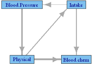
Table 4 shows the canonical correlations between the groups of variables among the post-pubertal subjects in NGHS cohort. These are all females within the age group 9 to 21 years, and only the observations after their Tanner stage II visit are used. The significant correlations are marked with *. Age is included in all models as a covariate; however, the causality network is drawn without the ‘Age’ node. Here we have a large cohort with complete observations, which may be the cause of the small correlations with significant test results. Consequently, the Granger network presented in Figure 1 is well connected, but most of the corresponding correlations are low. Regardless, most of the causalities depicted in Figure 1 are intuitive: change in intake is causing change in blood pressure and blood chemistry; change in physical parameters is causing change in intake and blood chemistry. Forward causality of blood pressure on physical variables is unexpected, as is the causality between intake and the physical variables. Another notable feature of the network is the lack of causality between blood chemistry and blood pressure, which suggests that the dependence is explained through other nodes.

Table 4: Cannonical correlations of the groups of variables in FLS postpubartal boys cohort with the response group in rows and causing groups on columns.’*’ indicates significant p value at 5% level of significance.

  

    
 
    
Physical
    
Blood. Pressure
    
Blood. chem
    
Intake
    
AGE
  
  

    
Physical
    
NA
    
0.3251
    
0.6688*
    
0.1875
    
0.2404
  
  

    
Blood. Pressure
    
0.5157
    
NA
    
0.5245
    
0.5864*
    
0.3936
  
  

    
Blood. chem
    
0.5169
    
0.6070
    
NA
    
0.4766
    
0.5298
  
  

    
Intake
    
0.1684
    
0.3248
    
0.5281
    
NA
    
0.0047
  

Table 4:  Cannonical correlations of the groups of variables in FLS postpubartal
boys cohort with the response group in rows and causing groups on columns.’*’
indicates significant p value at 5% level of significance.

Close

Figure 1: Granger causality network among the NGHS participants during their post-pubertal period. Edge thickness is proportional to the canonical correlation between the two groups.

    

    

    Figure 1:  Granger causality network among the NGHS participants during
their post-pubertal period. Edge thickness is proportional to the canonical
correlation between the two groups.
    
    

Close

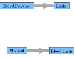
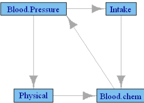
Table 4 presents the canonical correlations among the groups defined in Table 1 in the male subgroup of FLS cohort. Here also, Tanner stage II was used to define the pubertal stage. Only the postpubertal data are used to define the subgroup, and Age is included in all models as a covariate. The final model included 115 male and 109 female subjects, with variable length of time of follow-up. Use of correlation requires multiple observations across time, but 12 of the female and 11 of the male subjects had 2 or fewer time points, thus reducing the effective sample size. Due to an insufficient number of subjects, few of the correlations are significant, although the actual values of the correlations are larger than those observed in the NGHS cohort. Both Figures 2 and 3 are generated by this analysis using the p values of the causality test and the value of the canonical correlations, respectively. The significant p-value network is naturally sparse with only two edges. Although the FLS cohort differs from the NGHS cohort, in gender composition and age range, it is interesting to note the similarities and differences between the networks. The causality in Figure 2 between physical variables and blood chemistry in participants in the FLS is also found in the NGHS network, but the causality between intake and blood pressure is reversed in direction. The canonical correlation network of the FLS participants presented in Figure 3 is similar to that in the NGHS network. Three of the causalities, namely blood pressure →physical parameters→ blood chemistry and food intake → blood chemistry, are also repeated in the NGHS network. Causality between physical parameters and intake is missing here, and the causality blood chemistry → blood pressure is the only new edge.

Figure 2: Granger causality network among FLS cohort boys using only the p values during their post-pubertal period. Edge thickness is proportional to the canonical correlation between the two groups.

    

    

    Figure 2:  Granger causality network among FLS cohort boys using only the p
values during their post-pubertal period. Edge thickness is proportional to the
canonical correlation between the two groups.
    
    

Close

Figure 3: Granger causality network among FLS boys using only cannonical correlations above 0.44. Edge thickness is proportional to the canonical correlation between the two groups.

    

    

    Figure 3:  Granger causality network among FLS boys using only cannonical
correlations above 0.44. Edge thickness is proportional to the canonical
correlation between the two groups.
    
    

Close

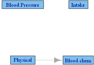
Table 5 shows the canonical correlations among the post-pubertal female population in the FLS cohort. Even though the canonical correlations are relatively larger compared to the NGHS cohort, none of the statistical tests reached significance, meaning the p-value induced network has no edges. The canonical correlation induced network, using the values above 0.44 is presented in Figure 4 and includes only one edge from physical parameters→ blood chemistry, which is common to all the networks.

Table 5: Cannonical correlations of the groups of variables in FLS postpubartal girls cohort with the response group in rows and causing groups on columns. ‘*’ indicates statistical significance at 5% level.

  

    
 
    
Physical
    
Blood. Pressure
    
Blood. chem
    
Intake
    
AGE
  
  

    
Physical
    
NA
    
0.4129
    
0.4867
    
0.1334
    
0.4442
  
  

    
Blood. Pressure
    
0.4229
    
NA
    
0.3111
    
0.2907
    
0.2894
  
  

    
Blood. chem
    
0.3278
    
0.2717
    
NA
    
0.1632
    
0.3146
  
  

    
Intake
    
0.1944
    
0.0732
    
0.2944
    
NA
    
0.0547
  

Table 5:  Cannonical correlations of the groups of variables in FLS postpubartal
girls cohort with the response group in rows and causing groups on columns. ‘*’
indicates statistical significance at 5% level.

Close

Figure 4: Granger causality network among FLS cohort post-pubertal girls using their cannonical correlations above 0.44.

    

    

    Figure 4:  Granger causality network among FLS cohort post-pubertal girls
using their cannonical correlations above 0.44.
    
    

Close

Discussion

Some of our findings align with biological intuition, notably the repeated patterns of food intake causing changes in blood chemistry, and physical parameters preceding change in blood chemistry. The repeated pattern of blood pressure causing physical parameters is a feature of our analysis that remains to be explored further through biological studies. Hypertension and BMI are other physical parameters whose has known association, though a causal direction has not been established.

Only in the subpopulation of post-pubertal boys did we find that blood chemistry affects blood pressure, and only in NGHS female subjects did we find that change in physical parameters precedes change in food intake. These directions can be explained as gender-specific effects. The interaction of blood pressure and food intake occurred in multiple networks with different directions. The biological basis of this interaction is not clear.

Regardless of the direction of interaction, the nodes ‘Physical parameters’ and ‘Blood chemistry’ remain the most connected nodes. Thus, these can be considered to be the central feature of this network. Implications of this connection can be used in strategies to manage overall health.

Conclusion

Our analysis highlights the difficulty of performing a data based multivariate causality inference in cohort study. The main limitations are the dimension of the model and sparseness of some of the variables. We did not use any imputation for this analysis, which led to many partial observations not being used. FLS data has 2567 subjects in total, but this analysis uses only 115 male and 109 female subjects. NGHS data, were reduced from 2380 subjects to 2250 subjects, however, 112 of them had only 2 or fewer post-pubertal visits. Regardless, there is a trend in causality structure that reinforces our prior understanding, and there are some new features that are worth further exploration.

The bigger goal behind such causality inference is to identify a “source of causality” among all the correlated collective nodes. In a way, irregularity in all the variables considered in our analysis define the complex phenotype ‘obesity’ rather than rather than just being associated. Therefore the process of management of obesity should have an impact on all the nodes of our network. Interdependence among them is likely to better guide us in developing a strategy to manage obesity. The most connected nodes in our analysis have been consistently the ‘physical parameters’ and ‘blood chemistry’. Therefore any health management strategy should focus on these nodes. This does not downplay the need to manage the other nodes. We only emphasize that starting management of physical parameters or blood chemistry will be more likely to produce a cascade effect on the other nodes, than the reverse. A successful health management should have a positive effect on all the variables considered here.

Acknowledgement

This study was supported by National Institutes of Health grant: U01HL101064, Bethesda, Maryland.

References

1. Olshansky SJ, Passaro DJ, Hershow RC, Layden J, Carnes BA, Brody J, et al. A potential decline in life expectancy in the United States in the 21st century. N Engl J Med. 2005; 352: 1138-1145.
2. Sinha R, Fisch G, Teague B, Tamborlane WV, Banyas B, Allen K, et al. Prevalence of impaired glucose tolerance among children and adolescents with marked obesity. N Engl J Med. 2002; 346: 802-810.
3. Sun SS, Grave GD, Siervogel RM, Pickoff AA, Arslanian SS, Daniels SR. Systolic blood pressure in childhood predicts hypertension and metabolic syndrome later in life. Pediatrics. 2007; 119: 237-246.
4. Sun SS, Liang R, Huang TT, Daniels SR, Arslanian S, Liu K, et al. Childhood obesity predicts adult metabolic syndrome: the Fels Longitudinal Study. J Pediatr. 2008; 152: 191-200.
5. Granger CWJ. Investigating causal relations by econometric models and cross-spectral meth- ods. Econometrica. 1969; 37: 424-438.
6. Mukhopadhyay ND, Chatterjee S. Causality and pathway search in microarray time series experiment. Bioinformatics. 2007; 23: 442-449.
7. Schäfer J, Strimmer K. An empirical Bayes approach to inferring large-scale gene association networks. Bioinformatics. 2005; 21: 754-764.
8. Zhu D, Hero AO, Cheng H, Khanna R, Swaroop A. Network constrained clustering for gene microarray data. Bioinformatics. 2005; 21: 4014-4020.
9. Dahlhaus R. Graphical interaction models for multivariate time series. Metrika. 2000; 51: 157-172.
10. Butte AJ, Bao L, Reis BY, Watkins TW, Kohane IS. Comparing the similarity of time-series gene expression using signal processing metrics. J Biomed Inform. 2001; 34: 396-405.
11. Salvador R, Suckling J, Schwarzbauer C, Bullmore E. Undirected graphs of frequency-dependent functional connectivity in whole brain networks. Philos Trans R Soc Lond B Biol Sci. 2005; 360: 937-946.
12. Winterhalder M, Schelter B, Hesse W, Schwab K, Leistritz L, Klan D, et al. Comparison of linear signal processing techniques to infer directed interactions in multivariate neural systems. Signal Processing. 2005; 85: 2137-2160.
13. Geweke JF. Measures of Conditional Linear Dependence and Feedback between Time Series Journal of the American Statistical Association. 1984; 79: 907-915.

Download PDF

Citation: Mukhopadhyay ND, Wheeler D, Sabo R and Sun SS. Multivariate Granger Causality Analysis of Obesity Related Variables. Austin Biom and Biostat. 2015;2(2): 1019. ISSN: 2378-9840

Home

Journal Scope

Online First

Current Issue

Editorial Board

Instruction for Authors

Submit Your Article

Contact Us