
Department of Mathematics and Computer science, Royal Military College of Canada, Canada
*Corresponding author: Shoucri RM, Department of Mathematics and Computer Science, Royal Military College of Canada, Kingston, ON, K7K 7B4, Canada
Received: September 23, 2014; Accepted: October 17, 2014; Published: October 20, 2014
Citation: Shoucri RM. Basic Relations between Ejection Fraction and ESPVR. Austin J Clin Cardiolog. 2014;1(5): 1029. ISSN 2381-9111
Heart Failure with normal or Preserved Ejection Fraction (HFpEF) is a subject that has received particular attention in the medical literature. In this study we show how the Ejection Fraction (EF) can be expressed as function of parameters describing the End-Systolic Pressure-Volume Relation (ESPVR), and the areas under the ESPVR, with new insight in some aspects of ventricular contraction. It is shown also that the Ejection Fraction (EF) is just one index of several indexes that can be derived from the parameters describing the ESPVR in order to assess the performance of the ventricles. Bivariate (or multivariate) analysis of indexes gives better segregation between cardiac cardiomyopathies. The ordinates of the ESPVR (units of pressure), and the areas under the ESPVR (units of energy) are sensitive parameters that reflect the state of the myocardium. Possible application of these results to the study of HFpEF is explained.
Keywords: End-Systolic pressure-volume relation; Ejection fraction; Cardiomyopathies; Ventricular contraction; Myocardium
It has been observed for some time that left (or right) ventricles presenting signs of cardiomyopathies can have normal Ejection Fraction (EF). It was first reported by Dumesnil et al. [1,2] that patients with aortic stenosis can have decreases in longitudinal shortening and wall thickening of the left ventricle, while the EF remains within normal limits because of the influence of intrinsic myocardial factors and/or left ventricular geometry. Several studies have since been published to explain the influence of intrinsic myocardial factors and ventricular geometry on EF, as well as other factors like the structure of the tissues of the myocardium, metabolism, ventricular suction and filling, preload and after load [3-6]. A related problem is the problem heart failure with normal or preserved ejection (HFpEF), it is estimated that half of the patients presenting symptoms of heart failure HF have preserved EF, defined as EF greater than 50% [7-9]. In this study we look at the way the EF is determined by parameters describing the End-Systolic Pressure-Volume Relation (ESPVR), these parameters include the ordinates of the ESPVR (units of pressure) and the areas under the ESPVR (units of energy). It is shown that new indexes derived from the ESPVR can also be used in assessing the ventricular contraction.
The ESPVR is the relation between the ventricular pressure Pm and volume Vm in the left (or right) ventricle when the myocardium reaches its maximum state of activation indicated by the elastance Emax (slope of the ESPVR). There have been several studies on the ESPVR [10-16] and its clinical applications, for a review see [12,16]. In a series of studies on the ESPVR published by the author, special attention was given to the introduction of the active force of the myocardium (also called isovolumic pressure Piso by physiologists) in the mathematical formalism describing the Pressure-Volume Relation (PVR) and the ESPVR in the ventricles [17-23]. In this study we review some basic relations that were derived to describe the ESPVR, as well as various relations to express the Stroke Volume (SV) (and consequently the EF =SV/Ved) in terms of the parameters describing the ESPVR and the areas under the ESPVR. We then show some new applications of these relations to clinical data published in the literature that give further evidence of the consistency of the mathematical formalism used. It is also shown that the EF is just one index of several new indexes derived from the ESPVR that can be used to assess the ventricular function. We finally indicate how the results obtained can open the way to new directions of research that can lead to new insight in the study of HFpEF.
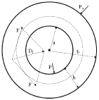
This section introduces some basic mathematical relations that are needed to describe the PVR in the ventricles. The left ventricle is represented as a thick-walled cylinder contracting symmetrically, as in previous publications [17-23]. A radial active force Dr (force per unit volume of the myocardium) is developed by the myocardium during the contraction phase (Figure 1). The active pressure on the inner surface of the myocardium (endocardium) is given by ∫ab Dr dr = Piso, where a: inner radius of the myocardium, b: outer radius of the myocardium. In a quasi-static approximation, we neglect inertia and viscous forces since they are relatively small. The equilibrium of forces on the surface of the endocardium can then be expressed in the form
Piso – P = E (Ved – V) (1)
Where P is the left ventricular pressure, the corresponding left ventricular volume is V, and Ved is the end-diastolic volume (the largest volume, when dV/dt = 0). The right-hand side of Eq. (1) represents the pressure on the endocardium resulting from the elastic deformation of the myocardium from Ved to V. When the elastance coefficient E reaches its maximum value Emax near end-systole (maximum state of activation of the myocardium), we can write Eq. (1) as follows
Pisom – Pm = Emax (Ved – Vm) (2)
In Eq. (2) Pisom, Pm and Vm are the corresponding values of Piso, P and V when Emax is reached, with Vm ≈ Ves the end-systolic volume (when dV/dt = 0). For simplicity we shall assume that the ventricular pressure P = Pm is constant during the ejection phase.
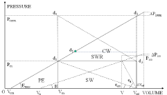
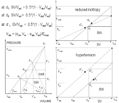
Equations (1) and (2) are represented graphically in a simplified way in Figure 2. The ESPVR is the relation between Pm and Vm when the myocardium reaches its maximum state of activation represented by Pisom, it is represented by the line d3Vom with slope Emax, mid-point d5 and volume axis intercept Vom. The line with slope E and volume axis intercept Vo in Figure 2 is an intermediate position. One can look at Eq. (1) in two ways:
Equations (1) and (2) can be split into two equations
P = E (V – Vo) (3)
Piso = E (Ved – Vo) (4)
and
Pm = Emax (Vm – Vom) (5)
Pisom = Emax (Ved – Vom) (6)
These relations indicate that there are three ways to represent the equation of the line with slope E (Eqs. (1), (3), (4)), as well as the equation of the line with slope Emax (Eqs. (2), (5), (6)) (see Figure 2).
Important information on the state of the myocardium can be obtained from the study of the relative position of the point d1 (corresponding to Pm) with respect to the mid-point d5 on the ESPVR (line d3Vom in Figure 2). This relative position can be described by the ratio Emax/eam (maximum ventricular elastance/maximum arterial elastance) and its relation to the stroke volume SV Ved – Vm (see Figure 2). We can distinguish the following cases:
In cases (b) and (c) an increase in pressure Pm causes a decrease in the stroke work SW, resulting in cardiac insufficiency.
Experimental verification of these results can be found in the works of Burkhoff et al. [12] (left ventricle) and Brimouille et al. [13] (right ventricle) for experiments on dogs, and in Asanoi et al. [15] for results on humans (left ventricle).
In the following new indexes derived from the ESPVR are used to classify the state of the myocardium as just described. It is also shown how SV and EF can be related to the indexes derived, and finally how the results obtained can be extended to the study of HFpEF. Experimental applications are based on clinical data taken from Borow et al [14] and from Asanoi et al [15]. In Borow et al [14] values of Emax and Vom are given for patients in control state and after injection of dobutamine. We have used the data of the first six groups in Table 1 of Borow et al [14], where also the dimensions of the left ventricle and the measurement of ESP (called Pm in our notation) are given. In Asanoi et al [15] values of Emax and Vom are given for three clinical groups of patients with EF ≥ 60%, 40% ≤ EF ≤ 59%, and EF ≤ 39%. We have also taken from Table 1 of Asanoi et al [15] the dimensions of the left ventricle and the values of ESP (called Pm in our notation). Notice that the dimensions of the variables used is immaterial if we use dimensionless ratios like Emax/eam.
Within the approximation used in this study, the areas under the ESPVR can be expressed as follows:
SW = Pm*SV (7)
CW = (Pisom – Pm)* SV/2 (8)
PE = Pm *(Vm – Vom) /2 (9)
SWR = SWx – SW (10)
TW = Pisom *(Ved – Vom)/2 (11)
Relation between TW and oxygen consumption was discussed in [22].
From these relations, one can derive the following relations for the stroke work (see [19,20]):
Emax/eam = 2*CW/SW (12)
SW/TW = 2*(Emax/eam)/(1 + Emax/eam)2 (13)
SW/PE = Emax/eam (14)
from which we can derive
SW2/4 = PE*CW (15)
These relations show the interrelation between SW with the areas under the ESPVR and the ratio Emax/eam. In particular Eq. (15) shows the balance of energy between SW, PE, and CW, that determines the value of SW.
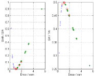
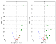
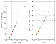
These relations are illustrated in Figs 3 to 6. Experimental data taken from Borow et al [14] are used in Figure 3. The property that Emax/eam → 1 when SV/(Ved –Vom) → 0.5 is verified (point d1 and d5 coincident in Figure 2), the right hand side shows the corresponding relation between Emax/eam and the EF which represents an approximation of the correct relation on the left hand side. Figure 4 represents the same relations for experimental data taken from Asanoi et al [15] for three clinical groups differentiated by their EF. From Figure 5 (left) we note that SWR/SW ≈ 0 for Emax/eam ≈ 1 as previously discussed (point d1 and d5 coincident in Figure 2) and from Figure 5 (right) we note that SW/TW ≈ 0.5 for Emax/eam ≈ 1 (SWx is half the total area TW). From Figure 6 (left) we note that SWR/SW ≈ 0 for SV/(Ved –Vom) ≈ 0.5, and Figure 6 (right) shows the corresponding relation between SWR/SW and SV/Ved. From Figure 5 (left) we notice that SWR/SW > 0.1 for Emax/eam > 2 corresponds to only normal EF, a similar observation can also be made from Figure 6 with SWR/SW > 0.1 for SV/(Ved – Vom) > 0.65. One can notice that the segregation of clinical groups in Figure 6 (left) is different from that shown in Figure 6 (right).
One can also derive the following relations (see Figure 2):
SV/(Ved – Vom) = (Pisom – Pm)/Pisom (16a)
from which we can derive the following expression for SV:
SV = (CW/TW)1/2 *(Ved – Vom) (16b)
It shows how SV (and consequently EF = SV/Ved) is influenced by the areas CW and TW under the ESPVR, as well as the intercept Vom of the ESPVR with the volume axis. We also have
SV = (Emax/eam) *(Vm – Vom) (16c)
Which is similar to the equation for SV derived in [24]. From Eq. (16c) one can also derive
SV = [Emax/(eam + Emax)]*(Ved – Vom) (16d)
Equations (16a) to (16d) show how the stroke volume SV (and the EF = SV/Ved) is determined by interacting parameters describing the ESPVR. When CW/TW = 1/4 (d1 and d5 coincide in Figure 2) we get from Eq. (16b) SV = (Ved – Vom)/2, which corresponds to Emax/ eam = 1.
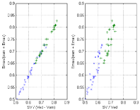
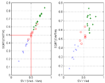
Eq. (16d) is illustrated with the experimental results shown in Figure 7, notice that SV/(Ved – Vom) → 0.5 when Emax/(eam + Emax) → 0.5, corresponding to Emax/eam =1 (d1 and d5 coincident in Figure 2). Similarly Eq. (16b) is illustrated with the experimental results shown in Figure 8, in this case we have CW/TW ≈ ¼ when SV/(Ved – Vom) ≈ 0.5.
One can finally derive the following relation between the parameters of the ESPVR:
Emax*Vom = evm*Vm – eam*Ved (17)
where evm = Pisom/SV. The relation between the parameters of the ESPVR given by Eq. (17) is illustrated in Figure 9.
We shall briefly show how the preceding results can be extended to the study of HFpEF, which approach is illustrated by the simplified drawing of Figure 10. The right side of Figure 10 (top) shows a case of normal ventricular contraction with d1 below the mid-point d5 on the ESPVR (solid line), and a case of depressed state of the myocardium due to reduced contractility with d1 above the mid-point d’5 on the ESPVR (dotted line, top), in both cases the EF = SV/Ved is the same and the detection of the anomaly can be done by using another indexes as shown from Fig. 3 to 8. like Emax/eam (Figure 10, left) or SV/(Ved – Vom) or (Pisom – Pm)/Pm or the areas under the ESPVR. Similar observation can be said for the case of hypertension in Fig. 10 (right, bottom) where the normal and hypertensive cases have the same EF = SV/Ved, the anomaly has to be detected by using other indexes as mentioned. Note that in real situations both Ved and Vm change [25], with the ratio (Ved – Vm) / Ved ≈ k nearly constant, which means that Vm ≈ (1 – k)Ved.
In cases of cardiomyopathies the ESPVR (and consequently Ved, Vm and Vom) have a tendency to shift to the right, Figure 10 is a simplified representation of a complex process.
Previous approaches to the study of the ESPVR [10,11,16] have focused on the part of this relation represented by the area PVA = PE + SW in Figure 2. An important contribution of the mathematical formalism used in this study is introduction of the active pressure Piso in the mathematical formalism describing the ESPVR and the appearance of a new area d1d2d3 (or CW) in Figure 2. The interrelation between the areas CW, SW and PE (having the units of energy) is an important aspect of the study of ventricular contraction. Only a few applications have been discussed in this study, they illustrate the rich collection of information that can be derived from the mathematical formalism used.
The results presented show that two-dimensional (bivariate) analysis of data is superior to univariate analysis. For instance in Figure 5 & 6, segregation of data with respect to the EF (right side) does not mean segregation with respect to other indexes. We have three clinical groups appearing around SV/(Ved – Vom) ≈ 0.5 and Emax/eam ≈ 1 that can be considered as critical values. How to obtain a combination of two indexes that can simultaneously segregate between different clinical cases still needs some study. In [23] we have indicated that dividing each clinical group by its standard deviation can achieve possible segregation; however this creates a problem of classification, given a new piece of data how to choose the standard deviation to classify it.
Future studies include the extension of the results of this study to the case of non-linear ESPVR, some preliminary results are given in [23]. Also the possibility of non-invasive implementation of these results by approximating the end-systolic ventricular pressure Pm with the peak carotid pressure or the peak blood pressure needs to be considered. Finally the extension of these results to cases of HFpEF as indicated in Figure 10 is a subject that deserves further attention.
This study has presented some relations that give new insight in the mechanics of ventricular contraction. We have shown how the Ejection Fraction (EF) is related to several parameters related to the ESPVR. Also a rich collection of indexes useful in clinical applications can be derived from the ESPVR. Bivariate (or multivariate) approach appears to be superior to univariate approach for the purpose of segregation and classification of clinical data, and can lead to interesting new results in the study of HFpEF.
Cross-section of a thick-walled cylinder representing the left ventricle.
P: Left Ventricular Pressure; Po: Outer Pressure (assumed zero), Dr: Active Radial Force/unit volume of the Myocardium; a: Inner Radius; b: Outer Radius, h = b – a: Thickness of the Myocardium.
PVR in the left ventricle represented by the loop Vedd2d1Vm in a normal ejecting contraction. The ESPVR is represented by the line d3Vom with midpoint d5 and slope Emax, the line with slope E corresponds to an intermediate position. The left ventricular pressure Pm is assumed constant during the ejection phase. The changes ΔPiso and ΔPisom correspond to changes ΔVed according to the Frank-Starling mechanism. The areas PE, SW, CW and SWR are defined in text. TW = PE + SW + CW is the total area under the ESPVR.
(left) Relation between Emax/eam = 2*CW/SW and SV/(Ved –Vom); (right) Relation between Emax/eam = 2*CW/SW and EF = SV/Ved. Experimental data from Borow et al [14], x control, + dobutamine.
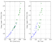
(left) Relation between Emax/eam = 2*CW/SW and SV/(Ved – Vom); (right) Relation Emax/eam = 2*CW/SW and EF = SV/Ved. Experimental data from Asanoi et al [15]. Data correspond to three clinical groups: (a) EF >= 60% ‘*’; (b) 40% < EF < 59% ‘o’; (c) EF < 40% ‘x’.
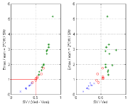
(left) Relation between SWR/SW and Emax/eam = 2*CW/SW; (right) Relation between SW/TW and Emax/eam = 2*CW/SW and EF = SV/Ved. Experimental data from Asanoi et al [15]. Data correspond to three clinical groups: (a) EF >= 60% ‘*’; (b) 40% < EF < 59% ‘o’; (c) EF < 40% ‘x’.
Relation between SWR/SW and SV/(Ved – Vom) (left side), and similar relation with EF = SV/Ved (right side). Experimental data from Asanoi et al [15]. Data correspond to three clinical groups: (a) EF >= 60% ‘*’; (b) 40% < EF < 59% ‘o’; (c) EF < 40% ‘x’.
Verification of Eq. (16d) (left side), and similar relation with the EF = SV/Ved (right side). Experimental data from Borow et al [14], x control, + dobutamine.
Verification of Eq. (16b) (left side), and similar relation with the EF = SV/Ved (right side). Experimental data from Asanoi et al [15]. Data correspond to three clinical groups: (a) EF >= 60% ‘*’; (b) 40% < EF < 59% ‘o’; (c) EF < 40% ‘x’.
Verification of Eq. (17). Experimental data from Asanoi et al [15]. Data correspond to three clinical groups: (a) EF >= 60% ‘*’; (b) 40% < EF < 59% ‘o’; (c) EF < 40% ‘x’.
(right) Normal physiological case with d1 below midpoint d5 (solid line); abnormal case with reduced contractility with d1 above midpoint d’5 (dotted line, top); abnormal case of hypertension with d’1 above midpoint d’5 (dotted line, bottom). Notice that the three cases have the same EF = SV/Ved. (left) ESPVR definitions as in Figure 2. The intercept with the horizontal axis Vdm is indicated as Vom in the text.
Austin Publishing Group is an emerging open access publisher specialising in Science, Technology and Medicine is dedicated to serve the biomedical community through its initiatives. Austin Publishing Group is an academic publisher with 100+ peer reviewed open access journals in various subjects such as biomedical, Pharma, Life Sciences, Environmental, Engineering and Management. Austin Publishing Group publishes Open Access eBooks providing free access to vast scientific literature.