Internal Fluctuations in a Population of Deer Mice with Hantavirus Infection

Abstract

We study the role of internal fluctuations and the thermodynamic limit in the population dynamics of deer mice, and describe the evolution of infected mice with Sin Nombre virus. This virus is the main cause of Hantavirus Pulmonary Syndrome (HPS) among humans in North America. In this way, we try to support those features observed in phenomenological models as the critical carrying capacity, K_c and the delay between population of mice and infected ones. We introduce the underlying processes, in particular the delayed maturation process, and derive from the master equation the mean field description for the thermodynamic limit. It matches the phenomenological model. Then we compare the model with the numerical Gillespie algorithm for the long-term phenomenon related to El Ni&nTilde;o southern oscillations. Internal fluctuations are able to drive the infection to extinction, mostly in the scenario of El Ni&nTilde;o, for both the transient and the steady state. We also study analitically the steady state. On the other hand, the thermodynamic limit plays the opposite role, and supports the infection. In general, we see how those features observed in the phenomenological description are where recovered both in the scenario related to La Ni&nTilde;a and in the thermodynamic limit.

Introduction

The population dynamics of deer mouse is central to the study of Hantavirus Pulmonary Syndrome (HPS), and is the subject of intense research since in 1993 deer mouse was identified as the host of SinNombre virus, which causes HPS [1].

Consequently, HPS cases are related to population of infected mice. We study this relation in terms of the basic epidemiological theory that suggests a link between HPS cases and contagion events. In particular humans get infected mainly through the contact with mice, or the inhalation of an aerosolized mixture of virus, feces and dried urine particles. Nowadays the mortality rate due to HPS is 40% [2].

At the same time contagion events are correlated with available resources. In the long term phenomena they depend on the climate variations and in particular on El Ni&nTilde;o southern oscillations.

On the other side, the virus remains inside the mouse without causing its death and propagating among mice horizontally, i.e., from mouse to mouse, mainly through direct contact [2]. In this direction several studies have pointed out how the number of infected mice is sensitive to El Ni&nTilde;o southern oscillations. During adverse periods the population of mice drastically decreases and the virus may even disappear. While on the contrary, when conditions improve, there is a big increase of population, high enough to cause an outbreak of infection [2,3].

In order to study the infection in deer mice at long-term, several simple models have been proposed [4-6].

The first model corresponds to Abramson-Kenkre (AK model), and describes the dynamics in terms of 2 variables, susceptible and infected mice [4]. The fundamental parameter of the model is the carrying capacity, K, that accounts for the amount of resources available for mice, and which value depends on the different scenarios related to El Ni&nTilde;o southern oscillations. When the scenario corresponds to El Ni&nTilde;o the amount of resources is high and consequently K increases, together with the population. In this case when K is bigger than a critical value, K_c, the infection spreads. While in La Ni&nTilde;a period, there are less resources and the scenario is related to a low value of K, and consequently the decrease in the number of mice. If K goes under K_c, the infection disappears.

In a new model, developed by the authors, we introduce a slightly different scheme to take into account a division in terms of age [5]. It is based on field studies that claim young mice do not contract the virus [7,8]. The model has 3 variables: young mice, susceptible adults and infected adults. It shows a characteristic time given by the maturation term, T, which produces a delay in both the outbreak and disappearance of infection in relation with the population of mice.

These phenomenological models are also extended to other climatic variations as the climate change mainly through the amount of available resources. An estimation of those resources, described by K, is crucial for the prediction and control of infection in areas where climate change is significant. As for El Ni&nTilde;o, good conditions are correlated with outbreaks while bad conditions are correlated with the reduction or the eradication of the infection.

While these models are deterministic, real systems are discrete and the number of related mice finite. This approach requires a better description in order to see the relevance of internal fluctuations and its relation with phenomenological models [9-11]. In particular, if those feature seen before for the phenomenological model in the long-term are supported by a more fundamental description [5].

In section II we consider the analytical approach given by the master equation. After that, in section III, we compare it with the exact numerical description for both above and below the thermodynamic limit. The numerical description is introduced by the modified Gillespie algorithm that considers non-markovian processes. In section IV, we first study fluctuations in the steady state with a perturbative method (subsection IV A) and later numerically with the modified Gillespie algorithm (subsection IV B). We also compare both approaches. Finally, conclusions summarize the results.

Analytical Results

Due to the stochasticity of the system, one has to rely on statistics and try to determine in a more solid description those features already seen in the phenomenological description. We first start writting down a general approach corresponding to the master equation. It describes the temporal evolution for the probability of the variables. In particular, we work with 3 variables: young mice, Y, susceptible adults, S, and infected adults, I. In compact form they look as following:

X = (Y, S, I) and X’ = (Y', S', I’)

$\frac{dP(X,t)}{dt}={\displaystyle \sum _{X^{\text{'}}}({\omega }_{X,X^{\text{'}}}}P(X^{\text{'}},t)-{\omega }_{X^{\text{'}},X}P(X,t))\text{ (1)}$

In our case, the master equation is built on several processes that account for the different ingredients introduced in [5]. They are represented through the transition rates,${\omega }_{X,X^{\text{'}}}$ and ${\omega }_{X^{\text{'}},X}$ , and consist in births, deaths, competition, contagion and maturation. They are all markovian processes except the maturation that lasts a finite time.

• Maturation

$Y\underset{\tau }{\to }S\text{ (2)}$

In order to go further and be able to derive the master equation, it is necessary to study in depth the maturation process. In this way, we divide it into more manageable sub processes.

Among them, the first sub process corresponds to a birth. Second, a period that describes the time mouse overcomes youth, T. And third, how mouse becomes adult, Y → S. The probability of the whole process is described as follows.

${\displaystyle \sum _{Y\text{'},S\text{'},I^{\text{'}}}P(Y,S,I,t+\Delta t;Y+1,S-1,I,t;\Gamma ;{\Upsilon }_{Y\text{'},S\text{'},I^{\text{'}}}})\text{ (3)}$

We analyze each process in a more precise and mathematical form [12].

The probability starts with the summation of all possible initial states corresponding to births (Y ', S ', I ' ) . This probability is represented by ${\Upsilon }_{Y\text{'},S\text{'},I^{\text{'}}}$, and corresponds to the following expression:

$P({\Upsilon }_{Y^{\text{'}}{S}^{\text{'}}{I}^{\text{'}}})=b(S^{\text{'}}+R^{\text{'}}+(Y^{\text{'}}-1))\Delta tP(Y^{\text{'}},S^{\text{'}},I^{\text{'}},t-\tau )$

Once the mouse is born it enters in the maduration period, represented by G. It describes how the mouse becomes adult and approached by e^-?t, where t is the maduration period and ? the difficulty to passing from youthhood to adulthood.

Finally, when the mouse arrives at (Y + 1, S - 1, I, t) it becomes a susceptible adult (Y, S, I, t + Δt). This last stage always happens when the other conditions fulfill.

At this point, we are able to write down the master equation in a more suitable form. In particular, we present it in terms of creation and destruction operators.

$\begin{array}{l}\text{Ef(X,t)=f(X+1,t) }\\ {\text{E}}^{\text{-1}}\text{(X,t)=f(X-1,t) (4)}\end{array}$

The final master equation for all the processes [5,9], reads as follows.

$\begin{array}{l}\frac{dP}{dt}=(E_Y^{-1}-1)b(Y+S+I)P+(E_Y-1)cYP\\ +(E_S-1)cSP+E_I-1)cIP\\ +(E_Y-1)\frac{1}{2k}Y(Y-1+S+I)P\\ +(E_S-1)\frac{1}{2k}S(Y+S-1+I)P\\ +(E_I-1)\frac{1}{2k}I(Y+S+I-1)P\\ +(E_s{E}_I^{-1}-1)aSIP\\ +(E_S^{-1}{E}_Y-1){\displaystyle \sum _{Y^{\text{'}}{S}^{\text{'}}{I}^{\text{'}}}P(Y,S,I,t/\Gamma ;{\Upsilon }_{Y^{\text{'}}{S}^{\text{'}}{I}^{\text{'}}})}\\ e^{-\gamma \tau }b(S^{\text{'}}+I^{\text{'}}+(Y^{\text{'}}-1))P(Y^{\text{'}},S^{\text{'}},I^{\text{'}},t-\tau )\text{ (5)}\end{array}$

This expression describes the time evolution for the probability of the 3 variables (Y,S,I). However, the set of equations is not closed and cannot be solved directly. On the other hand it is possible to get insight looking at different moments. In particular we study the first moment. For this case we approximate $\overline{X_i{X}_j}=\overline{X_i}\overline{X_j}$, where i and j indicate the different variables

$\frac{d\overline{Y}}{dt}=b\overline{M}-c\overline{Y}-\frac{\overline{Y}(\overline{M}-1)}{2k}-b{e}^{-\lambda t}(\overline{M}(t-\tau )-1)\left(6\right)$

$\frac{d\overline{S}}{dt}=b{e}^{-\lambda \tau }(\overline{M}(t-\tau )-1-c\overline{S}-\frac{\overline{S}(\overline{M}-1)}{2k}-a\overline{S}\overline{I}\left(7\right)$

$\frac{d\overline{I}}{dt}=-c\overline{I}-\frac{\overline{I}(\overline{M}-1)}{2k}+a\overline{S}\overline{I}\left(8\right)$

This new description corresponds to the mean values of the probability. We can go a step further and consider the thermodynamic limit as a particular case. If N → ∞ and Ω → ∞ keeping constant N/Ω, and considering the density instead of the number of mice, the remaining expressions are

$\frac{d{M}_Y}{dt}=bM-c{M}_Y-\frac{M_{Y}M}{K}-b{e}^{-\lambda \tau }M(t-\tau )\text{ (9)}$

$\frac{d{M}_{As}}{dt}=b{e}^{-\lambda \tau }(t-\tau )-c{M}_{As}-\frac{M_{As}M}{K}-a{M}_{As}{M}_{Ai}\text{ (10)}$

$\frac{d{M}_{Ai}}{dt}=-c{M}_{Ai}-\frac{M_{Ai}M}{K}-a{M}_{As}{M}_{Ai}\text{ (11)}$

Where, Y As Ai Y As Ai $M_Y=\frac{\overline{Y}}{\Omega },M_S=\frac{\overline{S}}{\Omega },M_I=\frac{\overline{I}}{\Omega },andM=M_Y+M_S+M_I$ Ù Ù Ù Parameters do not change, while a=aΩ and K=2k/Ω.

This mean field approach is in consonance with the phenomenological model introduced in [5]. In this case, the phenomenological description and its features are capture in the thermodynamic limit. However, we still do not know if those features are also valid in regions where internal fluctuations are significant.

Numerical Studies Comparision

The delayed Gillespie algorithm has been studied recently [13- 15]. Following the exact scheme developed by Cai, we have adapted it to our system by introducing a probability in the process that governs the transition to adulthood.

To study the role of fluctuations we identify two different scenarios depending on climatic conditions as the El Ni&nTilde;o southern oscillations [5]. Scenario A corresponds to favorable conditions (El Ni&nTilde;o) for the increase of population and the subsequent outbreak of infection. And scenario B where the conditions are harsh (La Ni&nTilde;a), and consequently the number of mice decrease together with the infection.

We will describe the system in both, in and out the thermodynamic limit. However, computational capabilities constrain our simulations to real domain (finite Ω). In order to get the thermodynamic limit we introduce fluctuations in the number of infected mice i.e., mice coming from adjacent niches. We introduce these fluctuations as a minimum source of infected mice.

A. Scenario A

In scenario A, the phenomenological model corresponds to K > K_c, is favorable to the increase of population [4,5]. As the virus spreads among adults, there is a delay between the population growth generated by the increase of youth, and the infection, which occurs when youth mice become adults. It is given by the maturation time, t, and characterizes the system [5]. We see how the evolution of the system comes into 2 different and consecutive time intervals. First, from (0, τ), the system evolves towards the absence of infection, and second, in (τ, ∞), the system evolves towards the outbreak of infection.

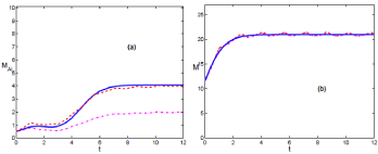
In (Figures 1a & b), we see the evolution of the mean value for those realizations above (dashed (red) line) and below thermodynamic limit (dash-dotted (magenta) line). In (Figure 1a), for the case of infected mice, the dash-dotted line does not follow the phenomenological model (solid (blue) line). It is due to the 0 absorbent state, reachable mainly in the interval (0, τ). In this scenario infection can disappear, and the outbreak of infection may not happen.

Figure 1: (Color online) Comparison of the temporal evolution for the phenomenological model in solid (blue) line and the mean value of realizations, in dash-dotted (magenta) line below the thermodynamic limit, while the dashed (red) line above it. Both set of realizations are obtained from the modified Gillespie algorithm. It describes scenario A. In (a) & (b), it is depicted M and M respectively. The carrying capacity is K = 15. K > K_c.

    

    

    Figure 1:  (Color online) Comparison of the temporal evolution for the phenomenological model in solid (blue) line and the mean value of realizations, in dash-dotted (magenta) line below the thermodynamic limit, while the dashed (red) line above it. Both set of realizations are obtained from the modified Gillespie algorithm. It describes scenario A. In (a) & (b), it is depicted M and M respectively. The carrying capacity is K = 15. K > Kc.
    
    

Close

The dashed (red) line corresponds to the thermodynamic limit, and evolves in consonance with the phenomenological description. In this case the absence of infection is not reachable. For the period (τ, ∞), the system evolves towards the outbreak of infection.

B. Scenario B

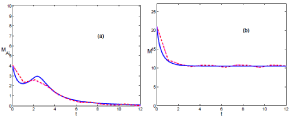
When climatic conditions are harsh, the phenomenological model is described by K < K_c, and the population decreases (see Figures 2a & b) following general trends [4,5]. The infection tends to disappear after a period of persistence given by the maturation time (see Figures 2a) [5]. This persistence is a serious thread that could lead to HPS cases.

In this scenario, (Figures 2a & b), fluctuations do not play any fundamental role since realizations evolve from finite values of infected mice in (0, τ) towards the lack of infection in the interval (τ, ∞), and both kind of realizations, below and above the thermodynamic limit fit qualitatively well with the phenomenological model.

It is also worth mentioning how the evolution of the number of mice in regimes, scenario A (Figure 1b) and B (Figure 2b), and the phenomenological model fit well and are described by the logistic equation [5].

Figure 2: (Color online) Comparison of the temporal evolution as in figure 1 for scenario B. Both situations, above and below the thermodynamic limit, evolve together. The carrying capacity takes the following value, K = 7.5. K < K_c.

    

    

    Figure 1:  (Color online) Comparison of the temporal evolution as in figure 1 for scenario B. Both situations, above and below the thermodynamic limit, evolve together. The carrying capacity takes the following value, K = 7.5. K < Kc.
    
    

Close

Steady State

In this section we study the probability density for the steady state in scenario A. First we introduce the analytical perturbative method and later we study numerically the steady state through the modified Gillespie algorithm. Finally, we compare both approaches.

A. Analytical approach

It is possible to develop a stochastic model based on the mean field description from which we can derive an approximation to the stationary probability for infected mice [9]. Let us decompose M in its steady mean value and its internal fluctuations: M + δM.

$M(t)=K(b-c)+\delta M(t)$ (12)

Where δM (t) is a random variable whose probability is given by the following expression with a white noise,ξ . [9].

$\frac{d\delta M(t)}{dt}=-(b-c)\delta M+\sqrt{2Kb(b-c)\xi (t)}$ (13)

$\begin{array}{l}<\delta M>=0\\ <{(}^{\delta }>=Kb\\ <\delta M(t)\delta M(t^{\text{'}})>=Kb{e}^{-(b-c)\left|t-t^{\text{'}}\right|}\text{ (14)}\end{array}$

We start from the mean field description (see equations. 9,10 and 11), and consider that δM is independent of δM (t-τ). Through some calculations, we arrive at a stochastic description for MAi.

$\frac{d{M}_{Ai}}{dt}=(aK(b-c)e^{-\lambda \tau }-b)M_{Ai}-a{M}_{Ai}^2-M_{Ai}\delta Z\text{ (15)}$

$\begin{array}{l}<\delta Z>=0\\ <{(}^{\delta }>=C^2\\ <\delta Z(t)\delta Z(t^{\text{'}})>=C^2{e}^{-(b-c)\left|t-t^{\text{'}}\right|}\left(16\right)\end{array}$

$C^2=Kb({(K^{-1}-a)}^2+\frac{a^2{R}^2}{c(2b-c)}+a(K^{-1}-a)(c(1-e^{-\lambda \tau })(\frac{1}{c}+\frac{1}{(2b-c)}$               (17)

This is a stochastic equation with colored noise. The approximate Fokker-Planck equation [16,17] which describes the process is the following one.

$\begin{array}{l}\frac{\partial P(M_{Ai},t)}{\partial t}=-\frac{\partial }{\partial M_{Ai}}G(M_{Ai})P(M_{Ai},t)+\frac{\partial }{\partial M_{Ai}}g(M_{Ai})\\ \frac{\partial }{\partial M_{Ai}}g(M_{Ai})D(M_{Ai})P(M_{Ai},t)\end{array}$               (18)

Where the different terms in the stochastic equation correspond to:

$G(M_{Ai})=(aK(b-c)e^{-\lambda \tau }-b)M_{Ai}-a{M}_{Ai}^2\text{ (19)}$

$g(M_{Ai})=-M_{Ai}$               (20)

$D(M_{Ai})=\frac{C^2}{(b-c)(b-c+a{M}_{Ai})}$               (21)

Now we look for the stationary probability density of M_Ai, considering that the boundary condition at ∞ is natural. N corresponds to the normalization constant.

$\begin{array}{l}P(M_{Ai})=N(1+\frac{a}{(b-c)}{M}_{Ai})\\ M_{Ai}(-1-\frac{b{(b-c)}^2}{c}+\frac{a(b-c){(b-c)}^2{e}^{-\lambda \tau }K}{c})\\ {\text{ e}}^{\text{-}\frac{(b-c)e^{-\lambda \tau }(a{M}_{Ai}^2(2a(-b+c)K+e^{\lambda \tau }(4b-2c+a{M}_{Ai})))}{2c{M}_{Ai}}}\end{array}$ (22)

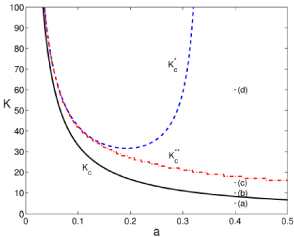
We see how the stationary probability density has a singularity at 0. In some cases it can be normalizable. In particular when K is above the curve $K_c=\frac{b{e}^{\lambda \tau }}{a(b-c)}.$

This curve is identified in (Figure 3) with the solid (black) line. There are also 2 more transitions. The region between the curves K_c and $K_c^{*}$ in dashed (blue) line still have a singularity at 0 together with a finite distribution for low values of infected mice. Above a second curve, $K_c^{**}$ in dash-dotted (red) line, a local maximum appears. And finally, for values above $K_c^{*}$ the singularity at 0 disappears.

Figure 3: Phase diagram for the theoretical stationary probability density of infected mice. We discuss it in terms of K and a, leaving constant the rest of parameters: b = 2, c = 0.6, ?=0.42 and, t=2. The solid (black) line corresponds to Kc, the dashed (blue) line to the transition given by $K_c^{*}$ and the dash-dotted (red) line to $K_c^{**}$ .Points labeled from (a) to (d) represent the values for the stationary probability density depicted in figure 4.

    

    

    Figure 3:  Phase diagram for the theoretical stationary probability density of
infected mice. We discuss it in terms of K and a, leaving constant the rest of
parameters: b = 2, c = 0.6, ?=0.42 and, t=2. The solid (black) line corresponds
to Kc, the dashed (blue) line to the transition given by $K_c^{*}$ and the dash-dotted (red) line to $K_c^{**}$
.Points labeled from (a) to (d) represent the values for the
stationary probability density depicted in figure 4.
    
    

Close

Thus, we find following the analysis developed in [9], that the steady state under internal fluctuations presents a general transition characterized by K_c. Behind it; internal fluctuations can drive the system to the 0 fixed point. However, as MAi increases together with K this chance decreases, K > K_c, and eventually the 0 fixed point becomes unreachable (above $K_c^{*}$ or a bottleneck to access the 0 fixed point for high values of K).

B. Numerical approach. Comparison

We study the numerical probability density for the steady state of scenario A with the modified Gillespie algorithm and compare it with the previous analytical results.

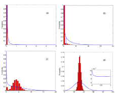
Since we only compute a small number of realizations (1000 realizations) in a finite time, we may describe partially the probability distribution. In (Figure 4) we see in (red) histograms the numerical approach. When K increases, the absorbent 0 fixed point becomes less reachable until it is finally unattainable (Figure 4 from (a) to (d)). At this point, (Figure 4d), the system is above the thermodynamic limit.

Figure 4: Stationary distribution density for infected mice corresponding to those parameters label in figure 3. We consider internal fluctuations both in the theoretical distribution in solid (blue) line and in the numerical (red) histogram. The phenomenological steady state is drawn with a vertical (blue) line. Displayed numerical distributions are taken over 1000 realizations at a finite time. The zoom in (d) shows the probability for the 0 absorbent state.

    

    

    Figure 4:  Stationary distribution density for infected mice corresponding to those parameters label in figure 3. We consider internal fluctuations both in the theoretical distribution in solid (blue) line and in the numerical (red) histogram. The phenomenological steady state is drawn with a vertical (blue) line. Displayed
numerical distributions are taken over 1000 realizations at a finite time. The zoom in (d) shows the probability for the 0 absorbent state.
    
    

Close

We now compare these results with theoretical probability distribution density in the steady state (solid (blue) line). In Figure 4, we show the spreading of the steady state due to internal fluctuations. For K < K_c there is no infection as we see in (a). However, from panels (b) to (d), K > K_c, we see how the system evolves towards a maximum for finite values of infection, and tends to leave unreachable the 0 fixed point. Following this evolution we see how in panel (c) the numerical description shows already a local maximum in contrast to the analytical description, where it has not appeared yet. The infection is more robust in the numerical distribution. Finally, in panel (d), we show how the system enters in the thermodynamic limit. Numerically, where the 0 fixed point becomes unreachable, and analytically, in those cases where there is a bottleneck that makes very difficult to reach the 0 fixed point.

In all, this suggests that the infection could get extincted in the stationary state out of the thermodynamic limit.

The mean field of these distributions coincides with the mean value of the phenomenological model when we consider the thermodynamic limit (vertical (blue) line).

Conclusions

Considering the finiteness and discreteness of our system, we have studied under the same conceptual framework as in [5], new analytical and numerical approaches in order to support those features observed in the phenomenological model for El Ni&nTilde;o southern oscillations. Throughout the article we have seen how in both, the temporal evolution and the steady state, the absent of infection is an absorbent state reachable out of the thermodynamic limit. In particular internal fluctuations are relevant in scenario A, unlike scenario B, where infection evolves to extinction. Mainly above the thermodynamic limit, we observe K_c and the delay among the total number of mice and those infected.

Acknowledgement

J. A. R. acknowledges support from grant BES-2008-003398.

References

1. Nichol S, Spiropoulou C, Morzunov S, Rollin P, Ksiazek T, Feldmann H, et al. Genetic identification of a hantavirus associated with an outbreak of acute respiratory illness. Science. 1993; 262: 914.
2. Yates TL, Mills JN, Parmenter CA, Ksiazek TG, Parmenter RR, Vande Castle JR, et al., BioScience. 2002; 52: 989.
3. Hjelle B, Glass GE. Outbreak of hantavirus infection in the Four Corners region of the United States in the wake of the 1997-1998 El Nino-southern oscillation. J Infect Dis. 2000; 181: 1569-1573.
4. Abramson G and Kenkre V. Spatiotemporal patterns in the Hantavirus infection. Phys Rev. 2002; 66.
5. Reinoso JA and Javier de la Rubia F. Spatial spread of the Hantavirus infection. Phys Rev. 2013; 87.
6. Kenkre V, Giuggioli L, Abramson G, and Camelo-Neto G. Effect of Predators of Juvenile Rodents on the Spread of the Hantavirus Epidemic. Eur Phys. J. 2007; 461.
7. Mills JN, Ksiazek TG, Peters C, Childs JE. Long-term studies of hantavirus reservoir populations in the southwestern United States: a synthesis. Emerg Infect Dis. 1999; 135-142.
8. Mills JN, Ksiazek TG, Ellis BA, Rollin PE, Nichol ST, Yates TL, et al. Patterns of association with host and habitat: antibody reactive with Sin Nombre virus in small mammals in the major biotic communities of the southwestern United States. Am J Trop Med Hyg. 1997; 56: 273-284.
9. Escudero C, Buceta J, de la Rubia FJ, Lindenberg K. Effects of internal fluctuations on the spreading of Hantavirus. Phys Rev. 2004.
10. Aguirre MA, Abramson G, Bishop AR, Kenkre VM. Simulations in the mathematical modeling of the spread of the Hantavirus. Phys Rev E Stat Nonlin Soft Matter Phys. 2002; 66: 041908.
11. G. Abramson. Mathematical modelling of Hantavirus: from the mean field to the individual level (edited by James T. Kelly. Progress in Mathematical Biology Research. 2007; 1-27.
12. Lafuerza LF and Toral R. Phys Rev. 2011; E 84, 051121.
13. Cai X. Exact stochastic simulation of coupled chemical reactions with delays. J Chem Phys. 2007; 126: 124108.
14. Bratsun D, Volfson D, Tsimring LS, Hasty J. Delay-induced stochastic oscillations in gene regulation. Proc Natl Acad Sci U S A. 2005; 102: 14593-14598.
15. Lafuerza LF and Toral R. Role of Delay in the Stochastic Creation Process. Phys Rev. 2011.
16. Fox RF. Functional-calculus approach to stochastic differential equations. Phys Rev A Gen Phys. 1986; 33: 467-476.
17. Fox RF. Uniform convergence to an effective Fokker-Planck equation for weakly colored noise. Phys Rev A Gen Phys. 1986; 34: 4525-4527.

Download PDF

Citation: Reinoso JA and de la Rubia JF. Internal Fluctuations in a Population of Deer Mice with Hantavirus Infection. Austin J Infect Dis. 2016; 3(1): 1019.

Home

Journal Scope

Online First

Current Issue

Editorial Board

Instruction for Authors

Submit Your Article

Contact Us